
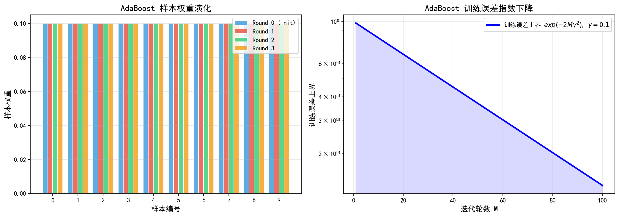
Misclassified samples gain weight after each round, while the upper bound on training error decreases with successive rounds under the weak-learning condition.
4.1 Overview and core idea
Yoav Freund and Robert E. Schapire first presented AdaBoost (Adaptive Boosting) as a conference paper in 1995 (EuroCOLT 1995) and published the full version in the Journal of Computer and System Sciences in 1997. It is the most classic and most influential member of the boosting family, and one of the most important algorithms in the history of machine learning.
The core idea comes down to “three cobblers working together are a match for Zhuge Liang”: train a series of weak classifiers iteratively — learners only slightly better than random guessing — and adapt the weight distribution over training samples so that later classifiers focus on the hard cases the earlier ones got wrong. Finally, combine the weak classifiers, weighted by performance, into one strong classifier.
How AdaBoost iterates:
- Initialize: give every sample equal weight, so the first weak classifier learns from the full dataset.
- Train: fit one weak classifier per round, and from its weighted error rate derive how much say that classifier gets (its weight $\alpha_m$).
- Update weights: raise the weight of misclassified samples and lower it for correctly classified ones, so the next weak classifier focuses on samples that haven’t been learned yet.
- Combine: put all weak classifiers to a weighted vote by $\alpha_m$ to get the final strong classifier.
  flowchart TD
    A["Initialize sample weights
w_i = 1/N"] --> B["Round m"]
    B --> C["Train weak classifier G_m under current weights"]
    C --> D["Compute weighted error rate ε_m"]
    D --> E["Compute weak classifier weight α_m"]
    E --> F["Update sample weights
misclassified samples gain weight"]
    F --> G{"Reached M rounds?"}
    G -->|No| B
    G -->|Yes| H["Weighted vote
G(x) = sign(Σ α_m G_m(x))"]
    H --> I["Output the final strong classifier"]
Why it matters: Freund & Schapire’s (1997) proof shows that as long as every weak classifier beats random guessing by a fixed advantage (error rate $\leq 1/2 - \gamma$ with $\gamma > 0$), AdaBoost’s training error falls exponentially with the number of rounds (see Section 4.6). The paper won the 2003 Gödel Prize. The result was a landmark in the theory of machine learning and gave boosting a firm theoretical footing.
4.2 Notation
Before the derivations, here is the notation used throughout this article:
| Symbol | Meaning | Notes |
|---|---|---|
| $(x_i, y_i), \ i=1,\dots,N$ | Training samples | $y_i \in \{-1, +1\}$ (binary labels) |
| $w_i^{(m)}$ | Weight of sample $i$ at round $m$ | $w_i^{(m)} > 0$; normalized in the algorithm so that $\sum_i w_i^{(m)} = 1$ (Sections 4.4 and 4.7 use the unnormalized version; the two differ by a constant factor) |
| $G_m(x)$ | Weak classifier trained at round $m$ | Outputs $G_m(x) \in \{-1, +1\}$ (hard classification) |
| $\alpha_m$ | Combination weight of the $m$-th weak classifier | $\alpha_m > 0$ when $\epsilon_m < 1/2$; the lower the error rate, the larger the weight |
| $\epsilon_m$ | Weighted error rate of the round-$m$ weak classifier | $\epsilon_m \in [0, 1]$ |
| $M$ | Total number of rounds (weak classifiers) | A preset hyperparameter |
| $G(x)$ | Final strong classifier | $G(x) = \operatorname{sign}\left(\sum_{m=1}^M \alpha_m G_m(x)\right)$ |
| $f_m(x)$ | Combined function at round $m$ (real-valued output) | $f_m(x) = \sum_{t=1}^m \alpha_t G_t(x)$ |
| $Z_m$ | Weight normalization factor at round $m$ | Keeps the normalized weights summing to 1 |
| $\gamma_m$ | The weak classifier’s advantage (edge) | $\epsilon_m = \frac{1}{2} - \gamma_m$, $\gamma_m > 0$; don’t confuse it with the sample margin in Section 4.7 |
| $\mathbb{I}(\cdot)$ | Indicator function | 1 when the condition holds, 0 otherwise |
| $K$ | Number of classes | Used in the multiclass extensions |
Convention: throughout this article the weak classifiers $G_m(x)$ output discrete labels $\{-1, +1\}$, which is what Discrete AdaBoost means. Later variants such as Real AdaBoost and SAMME.R use real-valued or probabilistic outputs.
4.3 Exponential loss and why it suits AdaBoost
AdaBoost optimizes the exponential loss:
$$L(y, f(x)) = \exp(-y \cdot f(x))$$Notation: $y \in \{-1, +1\}$ is the true label; $f(x)$ is the real-valued output of the combined classifier.
Why exponential loss suits AdaBoost
Look at how the loss behaves with respect to classification correctness:
- When $y \cdot f(x) > 0$ (correct): $L < 1$, and the larger $y \cdot f(x)$ — the more confident the call — the closer the loss to 0.
- When $y \cdot f(x) < 0$ (incorrect): $L > 1$, and the more negative $y \cdot f(x)$, the more lopsided the error, the more the loss grows — exponentially.
- When $y \cdot f(x) = 0$ (the decision boundary): $L = 1$.
  graph LR
    subgraph "How exponential loss behaves"
        A["y·f(x) > 0"] -->|correct| B["loss < 1
decays exponentially with confidence"]
        C["y·f(x) < 0"] -->|incorrect| D["loss > 1
grows exponentially with the size of the error"]
        E["y·f(x) = 0"] -->|decision boundary| F["loss = 1"]
    end
Exponential loss versus 0-1 loss
The theoretical elegance of AdaBoost is that exponential loss is an upper bound on the 0-1 loss:
$$\mathbb{I}\left(y f(x) \leq 0\right) \leq \exp\left(-y f(x)\right)$$(When $y f(x) \leq 0$ the right side is $\geq 1$; otherwise it’s $> 0$. The inequality therefore always holds.) Summing over the training set gives the starting point of Freund & Schapire’s (1997) training-error bound:
$$\sum_{i=1}^{N} \mathbb{I}\left(y_i f_M(x_i) \leq 0\right) \leq \sum_{i=1}^{N} \exp\left(-y_i f_M(x_i)\right)$$The left side counts misclassified training samples (a tie at $f_M(x_i) = 0$ counts as an error); the right side is the total exponential loss. So minimizing the exponential loss on the right also controls the training-error bound on the left. That is one of the central theoretical reasons AdaBoost works.
  graph TD
    A["Minimize exponential loss"] --> B["Bound the 0-1 loss from above"]
    B --> C["Training error falls exponentially"]
    C --> D["Final strong classifier"]
4.4 Deriving the weak classifier weight $\alpha_m$ (four steps)
At round $m$, AdaBoost picks a weak classifier $G_m$ and a weight $\alpha_m$ that minimize the exponential loss for that round:
$$(\alpha_m, G_m) = \arg\min_{\alpha, G} \sum_{i=1}^{N} w_i^{(m)} \exp(-\alpha \cdot y_i G(x_i))$$Here $w_i^{(m)} = \exp(-y_i f_{m-1}(x_i))$ is the sample weight determined by the combined classifier from the previous $m-1$ rounds — the weight distribution in the current objective. It doesn’t depend on $\alpha$ or $G$, so within this round it’s a constant; it differs from the normalized weight in the algorithm by a positive constant factor, which leaves the $\arg\min$ unchanged.
Step 1: split the objective by correct and incorrect classification
Since $y_i G(x_i) \in \{-1, +1\}$ (both are $\{-1, +1\}$ labels, so $+1$ when they agree and $-1$ when they don’t), the objective splits as
$$\sum_{i=1}^{N} w_i^{(m)} \exp(-\alpha y_i G(x_i)) = e^{-\alpha} \sum_{y_i = G(x_i)} w_i^{(m)} + e^{+\alpha} \sum_{y_i \neq G(x_i)} w_i^{(m)}$$Notation: $y_i = G(x_i)$ is the set of correctly classified samples; $y_i \neq G(x_i)$ is the set of misclassified ones.
Step 2: introduce the weight totals
Let
- $W_c = \sum_{y_i = G(x_i)} w_i^{(m)}$ (total weight of correctly classified samples)
- $W_e = \sum_{y_i \neq G(x_i)} w_i^{(m)}$ (total weight of misclassified samples)
- $W_{\text{total}} = W_c + W_e$ (total weight)
The objective becomes
$$e^{-\alpha} W_c + e^{+\alpha} W_e = (e^{-\alpha} - e^{+\alpha}) W_c + e^{+\alpha} W_{\text{total}}$$Step 3: choosing the optimal weak classifier
For any fixed $\alpha > 0$, since $e^{-\alpha} < e^{+\alpha}$, the coefficient on $W_c$, $(e^{-\alpha} - e^{+\alpha})$, is negative. Minimizing the whole expression is therefore equivalent to maximizing $W_c$, that is, minimizing $W_e$:
$$G_m = \arg\min_{G} \sum_{i=1}^{N} w_i^{(m)} \, \mathbb{I}\left(y_i \neq G(x_i)\right)$$Intuition: with $\alpha$ fixed, you should pick the weak classifier with the smallest weighted error. That’s exactly why AdaBoost passes the sample weights $w_i^{(m)}$ into WeakLearn each round — it makes the weak learner focus on the high-weight hard samples.
Step 4: differentiate with respect to $\alpha$
Substituting the optimal $G_m$ back and defining the weighted error rate
$$\epsilon_m = \frac{\sum_{i=1}^{N} w_i^{(m)} \, \mathbb{I}\left(y_i \neq G_m(x_i)\right)}{\sum_{i=1}^{N} w_i^{(m)}} = \frac{W_e}{W_{\text{total}}}$$the objective can be written as
$$L(\alpha) = W_{\text{total}} \left[ e^{-\alpha}(1 - \epsilon_m) + e^{+\alpha} \epsilon_m \right]$$Differentiate with respect to $\alpha$ and set the derivative to zero:
$$\frac{\mathrm{d}L}{\mathrm{d}\alpha} = W_{\text{total}} \left[ -e^{-\alpha}(1 - \epsilon_m) + e^{+\alpha} \epsilon_m \right] = 0$$$$e^{2\alpha} = \frac{1 - \epsilon_m}{\epsilon_m}$$Since $L(\alpha)$ is convex (its second derivative $W_{\text{total}}\left[e^{-\alpha}(1-\epsilon_m) + e^{\alpha}\epsilon_m\right] > 0$), this stationary point is the global minimum.
Final formula:
$$\boxed{\alpha_m = \frac{1}{2} \ln\left(\frac{1 - \epsilon_m}{\epsilon_m}\right)}$$Notation: $\alpha_m$ is the combination weight of the round-$m$ weak classifier; $\epsilon_m$ is the round-$m$ weighted error rate; $\ln$ is the natural logarithm.
What the formula means
| $\epsilon_m$ | $\alpha_m$ | Reading |
|---|---|---|
| $\epsilon_m \to 0$ (near-perfect) | $\alpha_m \to +\infty$ | The classifier gets an enormous say |
| $\epsilon_m = 0.1$ | $\alpha_m \approx 1.10$ | High weight |
| $\epsilon_m = 0.3$ | $\alpha_m \approx 0.42$ | Moderate weight |
| $\epsilon_m = 0.5$ (random guessing) | $\alpha_m = 0$ | No say; dropped |
| $\epsilon_m > 0.5$ (worse than chance) | $\alpha_m < 0$ | Negative weight in the formula (equivalent to using the prediction inverted); but standard AdaBoost.M1 stops outright once $\epsilon_m > 1/2$ (see Section 4.11) |
  graph LR
    subgraph "α_m as a function of error rate"
        A["ε_m → 0"] -->|near-perfect| B["α_m → +∞
enormous say"]
        C["ε_m = 0.5"] -->|random| D["α_m = 0
no say"]
        E["ε_m > 0.5"] -->|worse than chance| F["α_m < 0
used inverted"]
    end
4.5 The weight update and how it behaves
Once $G_m$ and $\alpha_m$ are set, the sample weights are updated so the next round focuses more on what this round got wrong:
$$w_i^{(m+1)} = \frac{w_i^{(m)} \cdot \exp\left(-\alpha_m \cdot y_i \cdot G_m(x_i)\right)}{Z_m}$$Notation: $Z_m$ is the normalization factor,
$$Z_m = \sum_{i=1}^{N} w_i^{(m)} \exp\left(-\alpha_m y_i G_m(x_i)\right)$$which ensures $\sum_{i=1}^{N} w_i^{(m+1)} = 1$. The minus sign matters: on a correct classification $y_iG_m(x_i)=+1$, so the weight is multiplied by $e^{-\alpha_m}$; on an error $y_iG_m(x_i)=-1$, so it’s multiplied by $e^{+\alpha_m}$.
Correct versus incorrect classification
Because $y_i G_m(x_i)$ depends on whether the classification was right:
Case 1: correct ($y_i = G_m(x_i)$, i.e. $y_i G_m(x_i) = +1$)
$$w_i^{(m+1)} = \frac{w_i^{(m)} \cdot e^{-\alpha_m}}{Z_m}$$Substituting $\alpha_m = \frac{1}{2} \ln\frac{1 - \epsilon_m}{\epsilon_m}$:
$$e^{-\alpha_m} = \sqrt{\frac{\epsilon_m}{1 - \epsilon_m}} < 1 \quad (\text{when } \epsilon_m < 0.5)$$Conclusion: correctly classified samples get multiplied by a factor $< 1$, so their weight drops.
Case 2: incorrect ($y_i \neq G_m(x_i)$, i.e. $y_i G_m(x_i) = -1$)
$$w_i^{(m+1)} = \frac{w_i^{(m)} \cdot e^{+\alpha_m}}{Z_m}$$$$e^{+\alpha_m} = \sqrt{\frac{1 - \epsilon_m}{\epsilon_m}} > 1 \quad (\text{when } \epsilon_m < 0.5)$$Conclusion: misclassified samples get multiplied by a factor $> 1$, so their weight rises.
The ratio between the two
The ratio of the new weight of an incorrect sample to that of a correct one is
$$\frac{w_{\text{wrong}}^{(m+1)}}{w_{\text{right}}^{(m+1)}} = \frac{w_{\text{wrong}}^{(m)}}{w_{\text{right}}^{(m)}} \cdot \frac{1 - \epsilon_m}{\epsilon_m}$$When $\epsilon_m$ is small (a very accurate weak classifier), the factor $\frac{1 - \epsilon_m}{\epsilon_m}$ is large, so the weight of misclassified samples is amplified sharply. When $\epsilon_m$ approaches 0.5, the factor approaches 1 and the adjustment is mild.
  graph TD
    subgraph "Weight update mechanism"
        A["sample i"] --> B{"G_m(x_i) = y_i?"}
        B -->|correct| C["weight × e^(-α_m)
weight drops"]
        B -->|incorrect| D["weight × e^(+α_m)
weight rises"]
        C --> E["next weak classifier
pays it less attention"]
        D --> F["next weak classifier
focuses on it"]
    end
4.6 The final classifier and the training-error bound (Freund & Schapire)
After $M$ rounds, AdaBoost’s final strong classifier is the weighted vote of all weak classifiers:
$$G(x) = \operatorname{sign}\left( \sum_{m=1}^{M} \alpha_m G_m(x) \right)$$Notation: $\operatorname{sign}(z) = +1$ if $z > 0$; $\operatorname{sign}(z) = -1$ if $z < 0$; when $z = 0$ either is allowed (usually $-1$ or $+1$).
The training-error bound
AdaBoost’s most striking theoretical result is its training-error bound. Suppose every weak classifier satisfies
$$\epsilon_m \leq \frac{1}{2} - \gamma_m$$where $\gamma_m > 0$ is how much better than chance that classifier is (its edge). Then the error of the final classifier $G(x)$ on the training set satisfies
$$\frac{1}{N}\sum_{i=1}^{N} \mathbb{I}\left(G(x_i) \neq y_i\right) \leq \prod_{m=1}^{M} Z_m = \prod_{m=1}^{M} 2\sqrt{\epsilon_m(1-\epsilon_m)} = \prod_{m=1}^{M} \sqrt{1 - 4\gamma_m^2} \leq \exp\left(-2 \sum_{m=1}^{M} \gamma_m^2\right)$$In particular, if all weak classifiers share a uniform edge $\gamma_m \geq \gamma > 0$ (each beats chance by at least $\gamma$), then
$$\boxed{\frac{1}{N}\sum_{i=1}^{N} \mathbb{I}\left(G(x_i) \neq y_i\right) \leq \exp\left(-2 M \gamma^2\right)}$$Notation: $M$ is the number of rounds; $\gamma$ is the smallest edge; $Z_m$ is the normalization factor from Section 4.5, computed with normalized weights.
Proving the theorem
The proof has three steps (see Freund & Schapire 1997; Li Hang, Statistical Learning Methods, §8.2).
Step 1: training error $\leq$ exponential loss. Write $f(x) = \sum_{m=1}^M \alpha_m G_m(x)$. By the inequality from Section 4.3, $\mathbb{I}\left(y f(x) \leq 0\right) \leq e^{-y f(x)}$:
$$\frac{1}{N}\sum_{i=1}^{N} \mathbb{I}\left(G(x_i) \neq y_i\right) \leq \frac{1}{N}\sum_{i=1}^{N} \exp\left(-y_i f(x_i)\right)$$Step 2: exponential loss $= \prod_m Z_m$. Starting from $w_i^{(1)} = 1/N$ and applying the update $w_i^{(m)} e^{-\alpha_m y_i G_m(x_i)} = Z_m w_i^{(m+1)}$ repeatedly:
$$\frac{1}{N}\sum_{i=1}^{N} \exp\left(-\sum_{m=1}^{M} \alpha_m y_i G_m(x_i)\right) = \sum_{i=1}^{N} w_i^{(1)} \prod_{m=1}^{M} e^{-\alpha_m y_i G_m(x_i)} = \left(\prod_{m=1}^{M} Z_m\right) \sum_{i=1}^{N} w_i^{(M+1)} = \prod_{m=1}^{M} Z_m$$Step 3: compute $Z_m$ and bound it. With normalized weights,
$$Z_m = (1-\epsilon_m) e^{-\alpha_m} + \epsilon_m e^{\alpha_m} = (1-\epsilon_m)\sqrt{\frac{\epsilon_m}{1-\epsilon_m}} + \epsilon_m \sqrt{\frac{1-\epsilon_m}{\epsilon_m}} = 2\sqrt{\epsilon_m(1-\epsilon_m)}$$Substituting $\epsilon_m = \frac{1}{2} - \gamma_m$ gives $Z_m = \sqrt{1 - 4\gamma_m^2}$. Then using $1 + x \leq e^x$ with $x = -4\gamma_m^2$, we get $\sqrt{1-4\gamma_m^2} \leq \sqrt{e^{-4\gamma_m^2}} = e^{-2\gamma_m^2}$, and multiplying over $m$ gives the result.
Steps 2 and 3 also show that the $\alpha_m$ AdaBoost picks is exactly the value that minimizes $Z_m$ — every round greedily minimizes the training-error bound.
What the theorem says
- Exponential decay: training error falls exponentially in the number of rounds $M$. Even with a tiny $\gamma$ (0.01, say — a weak classifier at 51% accuracy), enough rounds drive training error arbitrarily close to 0. Better still, training error can only take the values $0, \frac{1}{N}, \frac{2}{N}, \ldots$, so as soon as the bound $e^{-2M\gamma^2} < \frac{1}{N}$ — that is, $M > \frac{\ln N}{2\gamma^2}$ — training error is exactly 0 (with $N = 1000$ and $\gamma = 0.1$, $M > 346$ suffices).
- The weak-learning assumption: the theorem requires the weighted error rate of every round to be strictly below $1/2$, and for the bound to approach 0 the edge $\gamma_m$ must not creep toward 0 (a uniform lower bound $\gamma$, for instance). Note that this error rate is measured on a changing weighted distribution: as training proceeds, the weights concentrate on hard samples, so it gets harder and harder for the weak classifier to keep its edge, and in practice $\epsilon_m$ tends to rise round by round toward $1/2$.
- No need to know the edge in advance: unlike early boosting algorithms (Schapire’s 1990 recursive construction, Freund’s Boost-by-Majority), AdaBoost doesn’t need $\gamma$ ahead of time. Each round’s $\alpha_m$ adapts to the measured $\epsilon_m$, and that’s what “adaptive” means.
  graph TD
    A["Weak-learning assumption
ε_m < 0.5"] --> B["Each round yields an edge γ_m > 0"]
    B --> C["Training-error bound
≤ exp(-2Σγ_m²)"]
    C --> D["Larger M → exponential decay"]
    D --> E["Training error → 0"]
4.7 The statistical view: equivalence to minimizing exponential loss (Friedman et al. 2000)
In their landmark 2000 paper “Additive Logistic Regression: A Statistical View of Boosting,” Friedman, Hastie and Tibshirani reinterpret AdaBoost as forward stagewise additive modeling that minimizes the exponential loss.
The key insight
AdaBoost = forward stagewise additive modeling + exponential loss
Forward stagewise additive modeling
Consider the additive model
$$f_M(x) = \sum_{m=1}^{M} \beta_m g_m(x)$$Notation: $g_m(x)$ is the basis function (the weak classifier $G_m(x)$ in AdaBoost); $\beta_m$ is the coefficient (the $\alpha_m$ in AdaBoost).
The strategy is: at step $m$, optimize only the parameters of the newly added basis function, leaving the previous $m-1$ sets untouched:
$$(\beta_m, g_m) = \arg\min_{\beta, g} \sum_{i=1}^{N} L\big(y_i, f_{m-1}(x_i) + \beta g(x_i)\big)$$The equivalence under exponential loss
With $L(y, f) = \exp(-y f)$, this becomes
$$(\beta_m, g_m) = \arg\min_{\beta, g} \sum_{i=1}^{N} \exp\big(-y_i f_{m-1}(x_i) - \beta y_i g(x_i)\big)$$Letting $w_i^{(m)} = \exp(-y_i f_{m-1}(x_i))$ — exactly the weight AdaBoost defines — we get
$$= \arg\min_{\beta, g} \sum_{i=1}^{N} w_i^{(m)} \exp(-\beta y_i g(x_i))$$This is precisely the objective AdaBoost optimizes each round. Each AdaBoost update is therefore a step of coordinate descent on the exponential loss.
The population minimizer and the Bayes-optimal classifier
Over the population distribution, the minimizer of the exponential loss is
$$f^*(x) = \arg\min_{f(x)} \mathbb{E}[\exp(-Y f(x)) \mid X=x] = \frac{1}{2} \log \frac{P(Y=+1 \mid X=x)}{P(Y=-1 \mid X=x)}$$Notation: $f^*(x)$ is the population minimizer; $P(Y=+1 \mid X=x)$ is the posterior probability of the positive class; $\log$ is natural log.
That is half the log-odds. The Bayes-optimal decision rule agrees in sign with $f^*(x)$:
$$\arg\max_y P(Y=y \mid X=x) = \operatorname{sign}\left(f^*(x)\right)$$So by minimizing exponential loss, AdaBoost is really estimating the log-odds of the class probability, and in doing so it approaches the Bayes-optimal classifier.
An important caveat: limits of the statistical view
Wyner (2003), in “On Boosting and the Exponential Loss,” pushed back on the statistical view: any classifier $F$ that separates the training samples perfectly ($y_i F(x_i) > 0$) can minimize the exponential loss by multiplying itself by an arbitrarily large positive constant, which changes nothing about its predictions. Minimizing exponential loss alone therefore doesn’t guarantee generalization.
Schapire (2013) went further: understanding AdaBoost means looking not only at what it optimizes (exponential loss) but at how it optimizes — the dynamics of iterative reweighting, margin maximization and so on. Margin theory (Schapire et al., 1998) offers the other explanation: AdaBoost improves generalization by increasing sample margins, not merely by reducing training error.
Margin theory
A common observation: after AdaBoost’s training error hits 0, test error keeps falling as training continues. Neither training error nor model complexity (more rounds, more complex model) explains that. Schapire, Freund, Bartlett & Lee (1998) explained it in terms of margins.
Normalize the combined classifier’s output by its total weight and define the margin of sample $(x_i, y_i)$ as
$$\operatorname{margin}(x_i, y_i) = \frac{y_i \sum_{m=1}^{M} \alpha_m G_m(x_i)}{\sum_{m=1}^{M} \lvert \alpha_m \rvert} \in [-1, 1]$$A positive margin means a correct classification, and its magnitude reflects how decisive the vote was: a margin near 1 means nearly all weak classifiers (by weight) voted correctly.
Generalization bound: let $d$ be the VC dimension of the hypothesis class containing the weak classifiers. Then with probability at least $1-\delta$, simultaneously for all $\theta > 0$,
$$P_{\mathcal{D}}\left[y f(x) \leq 0\right] \leq P_{S}\left[y f(x) \leq \theta\right] + O\left(\sqrt{\frac{d \log^2(N/d)}{N \theta^2} + \frac{\log(1/\delta)}{N}}\right)$$where $f$ is the normalized combined output, $P_{\mathcal{D}}$ is the probability under the true distribution (the generalization error) and $P_S$ is the empirical proportion on the training set. This bound doesn’t depend on the number of rounds $M$: as long as most training samples have a large margin, generalization is guaranteed.
AdaBoost increases margins: Schapire et al. further showed that the fraction of training samples whose margin is at most $\theta$ after AdaBoost training satisfies
$$P_S\left[y f(x) \leq \theta\right] \leq 2^M \prod_{m=1}^{M} \sqrt{\epsilon_m^{1-\theta} (1-\epsilon_m)^{1+\theta}}$$When $\epsilon_m \leq \frac{1}{2} - \gamma$ and $\theta$ is small enough (below some multiple of $\gamma$), the right side falls exponentially in $M$. At $\theta = 0$ it reduces to the training-error bound above. In other words, once training error reaches 0, AdaBoost keeps pushing barely-correct samples toward larger margins, and that’s why test error can keep falling.
Controversy: margin theory isn’t settled. Breiman’s (1999) arc-gv algorithm achieves a larger minimum margin than AdaBoost yet generalizes worse. Reyzin & Schapire (2006) attribute this to arc-gv’s more complex base learners (deeper trees) and argue that what matters is the whole margin distribution, not just the minimum.
  graph LR
    A["AdaBoost training"] --> B["Training error ↓"]
    A --> C["Margin ↑"]
    B --> D["Exponential-loss minimization
Friedman et al. 2000"]
    C --> E["Better generalization
Schapire et al. 1998"]
    D --> F["Statistical explanation"]
    E --> F
4.8 AdaBoost variants
The AdaBoost family is large, with extensions for different task types (multiclass, regression) and different optimization strategies (real-valued output, probability estimation, robustness).
| Variant | Proposed by / year | Core idea | When to use |
|---|---|---|---|
| AdaBoost.M1 | Freund & Schapire (1997) | The original multiclass extension, requiring $\epsilon_m < 1/2$ | Multiclass, but the threshold is too strict |
| SAMME | Zhu, Zou, Rosset & Hastie (2009; technical report 2006) | A genuine multiclass AdaBoost, $\alpha_m = \log\frac{1-\epsilon_m}{\epsilon_m} + \log(K-1)$ | Multiclass ($K>2$); only needs accuracy better than $1/K$ |
| SAMME.R | Zhu et al. (2006 technical report version) | Real-valued updates from class probability estimates, faster convergence | Multiclass where probability estimates are available; removed from scikit-learn |
| AdaBoost.R2 | Drucker (1997) | Normalizes regression error and uses it to update weights | Regression |
| Real AdaBoost | Schapire & Singer (1999); probabilistic form given by Friedman et al. (2000) | Weak learners output real-valued confidence, $f_m(x) = \frac{1}{2}\log\frac{p_m(x)}{1-p_m(x)}$ | When weak learners can estimate class probabilities |
| Gentle AdaBoost | Friedman et al. (2000) | Newton-step optimization, smoother updates | Noisy data; more stable |
| LogitBoost | Friedman et al. (2000) | Minimizes the Bernoulli log-likelihood (logistic loss) rather than exponential loss | When probability interpretation matters |
| AdaBoost.RT | Shrestha & Solomatine (2006) | A threshold turns regression error into 0-1 error | Regression, adapting classification AdaBoost directly |
| BrownBoost | Freund (2001) | More robust to noise; allows training error slightly above 0 | Noisy labels |
| RobustBoost | Freund (2009) | Builds on BrownBoost; robust to label noise (implemented in MATLAB’s fitcensemble) | Noisy labels |
What SAMME changes
SAMME (Stagewise Additive Modeling using a Multi-class Exponential loss function) adds a $\log(K-1)$ term to $\alpha_m$:
$$\alpha_m = \log\left(\frac{1 - \epsilon_m}{\epsilon_m}\right) + \log(K - 1)$$where $\epsilon_m$ is the weighted multiclass error at round $m$. Sample weights update as $w_i \leftarrow w_i \exp\left(\alpha_m \mathbb{I}\left(c_i \neq G_m(x_i)\right)\right)$ followed by normalization ($c_i$ is the class of sample $i$), and the final classifier is $G(x) = \arg\max_k \sum_m \alpha_m \mathbb{I}\left(G_m(x) = k\right)$.
The key advantage: $\alpha_m > 0$ only when $\epsilon_m < 1 - \frac{1}{K}$, i.e. accuracy above the $1/K$ of random guessing. So SAMME only asks the weak classifier to beat chance, not to exceed 1/2 accuracy as AdaBoost.M1 does. At $K = 2$, $\log(K-1) = 0$ and $\alpha_m = \ln\frac{1-\epsilon_m}{\epsilon_m}$, exactly twice this article’s $\frac{1}{2}\ln$ form; the final classifier is identical, so SAMME reduces to standard AdaBoost.
SAMME.R’s real-valued update
SAMME.R uses the weak classifier’s class probability estimates $p_k^{(m)}(x)$ to compute a real-valued update:
$$h_k^{(m)}(x) = (K-1) \left( \log p_k^{(m)}(x) - \frac{1}{K} \sum_{k'=1}^{K} \log p_{k'}^{(m)}(x) \right)$$Notation: $h_k^{(m)}(x)$ is the real-valued update for class $k$ at round $m$; $p_k^{(m)}(x)$ is the probability the round-$m$ weak classifier assigns to class $k$.
In Zhu et al.’s experiments SAMME.R usually converges faster, but it requires the base learner to support probability estimates (predict_proba). According to scikit-learn’s maintainers (GitHub issue #26784), SAMME.R appeared only in the 2006 technical report, wasn’t included in the formally published journal version, and diverged in observed behavior; scikit-learn therefore deprecated it in 1.4, removed algorithm='SAMME.R' in 1.6, and removed the whole algorithm parameter in 1.8.
Real AdaBoost: real-valued output
Discrete AdaBoost’s weak classifiers output only $\pm 1$. Schapire & Singer (1999) allowed weak learners to output a real-valued confidence, and Friedman, Hastie & Tibshirani (2000) gave the class-probability version (Real AdaBoost):
- Initialize $w_i = 1/N$;
- For $m = 1, \ldots, M$:
- Train a classifier under weights $w_i$ and get the weighted class probability estimate $p_m(x) = \hat{P}_w(y = 1 \mid x) \in (0, 1)$;
- Set $f_m(x) = \frac{1}{2}\log\frac{p_m(x)}{1 - p_m(x)}$;
- Update $w_i \leftarrow w_i \exp\left(-y_i f_m(x_i)\right)$ and normalize;
- Output $G(x) = \operatorname{sign}\left(\sum_{m=1}^M f_m(x)\right)$.
Here $f_m(x)$ is exactly the pointwise solution to minimizing $\mathbb{E}_w\left[e^{-y f(x)} \mid x\right]$ under the current weighted distribution (the same derivation as the population minimizer in Section 4.7), so Real AdaBoost is likewise a forward stagewise algorithm under exponential loss. In practice $p_m(x)$ has to be clipped to $[\varepsilon, 1-\varepsilon]$ so that $f_m(x)$ doesn’t blow up.
  graph TD
    A["AdaBoost, binary"] --> B["AdaBoost.M1
multiclass extension"]
    A --> C["SAMME
a true multiclass generalization"]
    B --> D["ε_m < 1/2 is a high bar"]
    C --> E["ε_m > 1/K suffices
more practical for K>2"]
    A --> F["Real AdaBoost
probability estimates"]
    A --> G["Gentle AdaBoost
Newton step"]
    A --> H["LogitBoost
log-likelihood"]
    A --> I["AdaBoost.R2
regression version"]
AdaBoost.R2: boosting for regression
Drucker (1997) proposed AdaBoost.R2, the classic route from classification AdaBoost to regression. The idea: normalize the regression error and map it to a sample-weight update factor, so later weak learners focus on whatever the model currently fits worst.
The mechanism
Instead of the 0-1 error of the classification version, AdaBoost.R2 normalizes each sample’s regression error to $[0,1]$ and updates weights from those. With $G_m(x)$ the round-$m$ weak regressor, first compute the absolute error:
$$e_i^{(m)} = \lvert y_i - G_m(x_i) \rvert$$Then normalize by the largest error in this round:
$$D_i^{(m)} = \frac{e_i^{(m)}}{\max_j e_j^{(m)}}$$where $D_i^{(m)} \in [0,1]$. The closer $D_i^{(m)}$ is to 0, the better the current weak regressor predicts sample $i$; the closer to 1, the larger the error.
scikit-learn’s AdaBoostRegressor also supports three error shapes, all built on the normalized error $D_i^{(m)}$:
loss | Per-sample loss $L_i^{(m)}$ | What it does |
|---|---|---|
'linear' | $L_i^{(m)} = D_i^{(m)}$ | Default; error enters the weight update in linear proportion |
'square' | $L_i^{(m)} = \left(D_i^{(m)}\right)^2$ | Emphasizes large-error samples more |
'exponential' | $L_i^{(m)} = 1 - \exp\left(-D_i^{(m)}\right)$ | Exponential transform compressed into $[0,1)$ |
Updating the weights
First compute the current weak regressor’s weighted average loss:
$$\bar{L}^{(m)} = \sum_{i=1}^N w_i^{(m)} L_i^{(m)}$$If $\bar{L}^{(m)} \geq \frac{1}{2}$, the current weak regressor isn’t good enough; training typically stops or the regressor is dropped. Otherwise define
$$\beta_m = \frac{\bar{L}^{(m)}}{1 - \bar{L}^{(m)}}$$Since $\bar{L}^{(m)} < \frac{1}{2}$, we have $\beta_m \in (0,1)$. Then update the sample weights:
$$w_i^{(m+1)} = w_i^{(m)} \cdot \beta_m^{1 - L_i^{(m)}}$$and normalize so the weights sum to 1.
The formula looks counterintuitive at first: rather than multiplying large-error samples by a big number, it multiplies small-error samples by a smaller number:
- A well-predicted sample has $L_i^{(m)} \approx 0$, so its multiplier is about $\beta_m$ and its weight drops noticeably;
- A badly predicted sample has $L_i^{(m)} \approx 1$, so its multiplier is about 1 and its weight barely moves;
- After normalization, the large-error samples’ relative weight goes up.
Weak learner weights
The combination weight of the $m$-th weak regressor in the final prediction is
$$a_m = \ln\left(\frac{1}{\beta_m}\right)$$The smaller $\beta_m$ is, the lower the current weak regressor’s weighted average loss, hence the larger $a_m$ and the more influence it has.
The final prediction
AdaBoost.R2 outputs the weighted median of the weak regressors’ predictions. The formula below uses $\operatorname{WeightedMedian}$ for this operation.
$$G(x) = \operatorname{WeightedMedian}\left(\{G_m(x)\}_{m=1}^M,\ \{a_m\}_{m=1}^M\right)$$with $a_m = \ln(1/\beta_m)$. The weighted median sorts $\{G_m(x)\}$ ascending and finds the first position where the cumulative weight on the left reaches half the total. Using a median instead of a plain average limits how much any single aberrant weak regressor can move the final result.
Pseudocode
- Input: training set $D = \{(x_i, y_i)\}_{i=1}^N, y_i \in \mathbb{R}$, weak regression algorithm $\text{WeakRegressor}$, number of rounds $M$
- Initialize: $w_i^{(1)} = 1/N, \quad i = 1, \ldots, N$
- For $m = 1, 2, \ldots, M$ do:
- Train a weak regressor $G_m(x)$ under weights $w_i^{(m)}$
- Compute the absolute error $e_i^{(m)} = \lvert y_i - G_m(x_i) \rvert$
- Compute the normalized error $D_i^{(m)} = e_i^{(m)} / \max_j e_j^{(m)}$
- Convert $D_i^{(m)}$ to $L_i^{(m)}$ according to
loss - Compute the weighted average loss $\bar{L}^{(m)} = \sum_i w_i^{(m)} L_i^{(m)}$
- If $\bar{L}^{(m)} \geq 1/2$, stop adding weak regressors
- Compute $\beta_m = \bar{L}^{(m)} / (1 - \bar{L}^{(m)})$
- Update the sample weights $w_i^{(m+1)} = w_i^{(m)} \cdot \beta_m^{1 - L_i^{(m)}}$
- Normalize so that $\sum_i w_i^{(m+1)} = 1$
- Output: $$G(x) = \operatorname{WeightedMedian}\left(\{G_m(x)\},\ \{\ln(1/\beta_m)\}\right)$$
Implementation note: scikit-learn’s
AdaBoostRegressorfollows Drucker’s original: each round it resamples the training set with replacement under the current weights and trains the weak regressor on the resampled data, rather than passing the weights throughsample_weight.
Versus classification AdaBoost: classification AdaBoost uses exponential loss and 0-1 error, whereas AdaBoost.R2 uses relative error and a median combination, which is more robust to outliers in regression. scikit-learn’s
AdaBoostRegressordefaults toloss='linear'(a linear loss);loss='square'orloss='exponential'select other error measures.
4.9 Strengths, weaknesses and when to use it
Strengths
| Strength | Notes |
|---|---|
| Strong theory | Training error falls exponentially with the number of rounds, as long as weak classifiers beat chance |
| Resists overfitting | On low-noise data, test error often keeps falling after training error hits 0 (margin theory explains this; see Section 4.7); but there’s no guarantee — with heavy noise it will overfit |
| Little tuning needed | Weak classifiers are usually decision stumps (depth=1), so there are few hyperparameters |
| Implicit feature selection | The weight update focuses attention on important features and hard samples |
| General | Any weak learner that supports sample weights (sample_weight) can be plugged in |
| Cheap to train | Training costs $O(M \cdot T_{\text{weak}})$, where $M$ is the number of rounds |
| Interpretable | feature_importances_ shows which features matter most |
Weaknesses
| Weakness | Notes |
|---|---|
| Sensitive to noise | Mislabeled samples get reweighted again and again, become “hard samples,” and the model overfits the noise. Long & Servedio (2010) proved further that any boosting algorithm minimizing a convex margin loss (AdaBoost and LogitBoost included) faces data distributions where it learns perfectly without noise but degrades to chance once any small fraction of random label noise is added |
| Sensitive to outliers | Wrong labels or extreme values hurt performance badly |
| Needs weak classifiers better than chance | If the weighted error rate is $\geq 1/2$ (binary), $\alpha_m \leq 0$ and no further progress is possible, so AdaBoost.M1 stops early; if the weak classifier is too strong (training error 0), then $\alpha_m \to \infty$ and training also can’t continue |
| Nontrivial multiclass extension | AdaBoost.M1 demands error $< 1/2$, too strict for many classes |
| Can overfit | When weak classifiers are too complex (deep trees) or there are too many rounds |
| Mediocre on imbalanced data | May need cost-sensitive variants such as AdaC2 |
| Hard to parallelize | Weak classifiers must be trained in sequence; rounds depend on each other |
When to use it
- Baselines: a fast, effective baseline classifier to establish a performance reference
- Feature importance:
feature_importances_for feature selection and explanation - Binary classification: AdaBoost is particularly strong here
- Small to medium datasets: works well when the data aren’t too large (under $100{,}000$ samples)
- Interpretability: stumps give an intuitive combination of rules
- Ensemble comparisons: the classic baseline to compare other ensemble methods against
When not to use it
- High-noise datasets: with heavy label noise or outliers, AdaBoost keeps reweighting the noisy samples
- Large datasets: training time grows linearly with rounds, so it’s less efficient than XGBoost/LightGBM at scale
- High-dimensional sparse data: bag-of-words text classification, for instance, where linear models usually do better
- When calibrated probabilities matter: raw AdaBoost’s probability outputs are poor (SAMME.R improves this)
- Multiclass problems ($K > 2$): prefer SAMME over AdaBoost.M1
4.10 The sklearn API and key parameters
scikit-learn provides AdaBoostClassifier and AdaBoostRegressor.
AdaBoostClassifier API
| |
Note: from scikit-learn 1.2 on,
base_estimatoris renamedestimator. In recent versionsAdaBoostClassifierkeeps only the discreteSAMMEalgorithm;SAMME.Rin older docs or code is a deprecated path and shouldn’t be used in new projects.
Key parameters
estimator (base learner)
- Default:
DecisionTreeClassifier(max_depth=1)(a stump) - Requirements: must support sample weights (the
sample_weightargument) plus theclasses_andn_classes_attributes - Common choices: stumps, shallow trees (
max_depth2-5), linear-kernel SVM - Advice: the default stump is usually good enough; deeper trees add capacity but also overfitting risk
n_estimators (number of weak classifiers)
- Default: 50
- Role: the maximum number of boosting rounds
- Note: if some round’s weak classifier fits the weighted training set perfectly (weighted error 0), sklearn stops early and
len(clf.estimators_)may be less thann_estimators. Beyond that there’s no automatic early stopping on a validation set; usestaged_predict/staged_scoreto choose the number of rounds yourself - Tuning advice:
- Small datasets (under 1000 samples): 50-100
- Medium datasets: 100-500
- Tune jointly with
learning_rate: a smallerlearning_rateneeds a largern_estimators
learning_rate
- Default: 1.0
- Role: shrinkage applied to each weak classifier’s weight. In sklearn each round’s classifier weight becomes $\eta\,\alpha_m$, where $\eta$ is
learning_rate, and the sample-weight update also uses the shrunk $\eta\,\alpha_m$: $$w_i \leftarrow w_i \exp\left(\eta\,\alpha_m \mathbb{I}\left(y_i \neq G_m(x_i)\right)\right), \qquad G(x) = \arg\max_k \sum_m \eta\,\alpha_m \mathbb{I}\left(G_m(x) = k\right)$$ (sklearn implements SAMME, so $\alpha_m$ follows the SAMME formula.) Note: scaling all final vote weights by $\eta$ alone wouldn’t change any prediction.learning_ratehas an effect because it makes each round’s sample reweighting gentler, which changes how the subsequent weak classifiers are trained. - Intuition: it plays the role of a step size in gradient descent. A smaller rate takes more conservative steps and needs more rounds
- Tuning advice:
- The default 1.0 usually works
- If you see overfitting, try 0.1-0.5 and raise
n_estimators - Rule of thumb:
learning_rateandn_estimatorstrade off. With rate $\eta$ and rounds $M$, the usual guidance is $$\eta \times M \approx \text{const}$$
algorithm (removed)
| Version | Status |
|---|---|
| 1.3 and earlier | algorithm accepts 'SAMME' or 'SAMME.R' (default 'SAMME.R') |
| 1.4 | 'SAMME.R' deprecated |
| 1.6 | 'SAMME.R' removed; the algorithm parameter itself deprecated (only 'SAMME' left) |
| 1.8 and later | algorithm removed; passing it raises TypeError |
- In practice: don’t pass
algorithmin new code —AdaBoostClassifieris SAMME by default. When maintaining old code that usesSAMME.R, re-check metrics on a validation set after migrating, since SAMME and SAMME.R can give noticeably different results.
AdaBoostRegressor API (regression only)
| |
The loss parameter (regression only):
| Loss | Formula | Notes |
|---|---|---|
'linear' | $L_i = D_i$ | Default; error enters the weight update in linear proportion |
'square' | $L_i = D_i^2$ | Emphasizes large-error samples more |
'exponential' | $L_i = 1 - \exp(-D_i)$ | Bounded; grows more slowly with large errors than 'linear' |
where $D_i = \lvert y_i - G_m(x_i) \rvert / \max_j \lvert y_j - G_m(x_j) \rvert \in [0, 1]$ is the normalized error from Section 4.8. All three losses act on $D_i$, not on the raw error $\lvert y - f \rvert$.
Important attributes
| Attribute | Meaning |
|---|---|
estimators_ | The fitted weak classifiers |
estimator_weights_ | Weight of each weak classifier (SAMME formula, already scaled by learning_rate; for binary problems this is twice this article’s $\alpha_m$) |
estimator_errors_ | Weighted error rate $\epsilon_m$ of each weak classifier (in the regressor, the weighted average loss $\bar{L}^{(m)}$) |
feature_importances_ | Feature importance: impurity-based importance from each base learner, averaged with estimator_weights_ as weights |
classes_ | Class labels |
n_classes_ | Number of classes |
4.11 Pseudocode
Algorithm: AdaBoost (Discrete AdaBoost / AdaBoost.M1)
- Input: training set $D = \{(x_i, y_i)\}_{i=1}^N, y_i \in \{-1, +1\}$, weak learning algorithm $\text{WeakLearn}$, number of rounds $M$
- Initialize: $w_i^{(1)} = 1/N, \quad i = 1, \ldots, N$
- For $m = 1, 2, \ldots, M$ do:
- Normalize the weights: $p_i = w_i^{(m)} / \sum_j w_j^{(m)}$
- Call $\text{WeakLearn}$ with distribution $p$ to get the weak classifier $G_m(x)$
- Compute the weighted error rate: $$\epsilon_m = \sum_{i=1}^N p_i \, \mathbb{I}\left(y_i \neq G_m(x_i)\right)$$
- If $\epsilon_m > 1/2$, stop (the weak learner isn’t good enough)
- Compute the weak classifier weight: $$\alpha_m = \frac{1}{2} \ln\left(\frac{1 - \epsilon_m}{\epsilon_m}\right)$$
- Update the sample weights: $$w_i^{(m+1)} = w_i^{(m)} \cdot \exp\left(-\alpha_m \cdot y_i \cdot G_m(x_i)\right)$$
- Normalize so that $\sum_i w_i^{(m+1)} = 1$
- Output the final classifier: $$G(x) = \operatorname{sign}\left(\sum_{m=1}^M \alpha_m G_m(x)\right)$$
4.12 A from-scratch Python implementation, line by line
| |
4.13 Using sklearn and tuning it
| |