
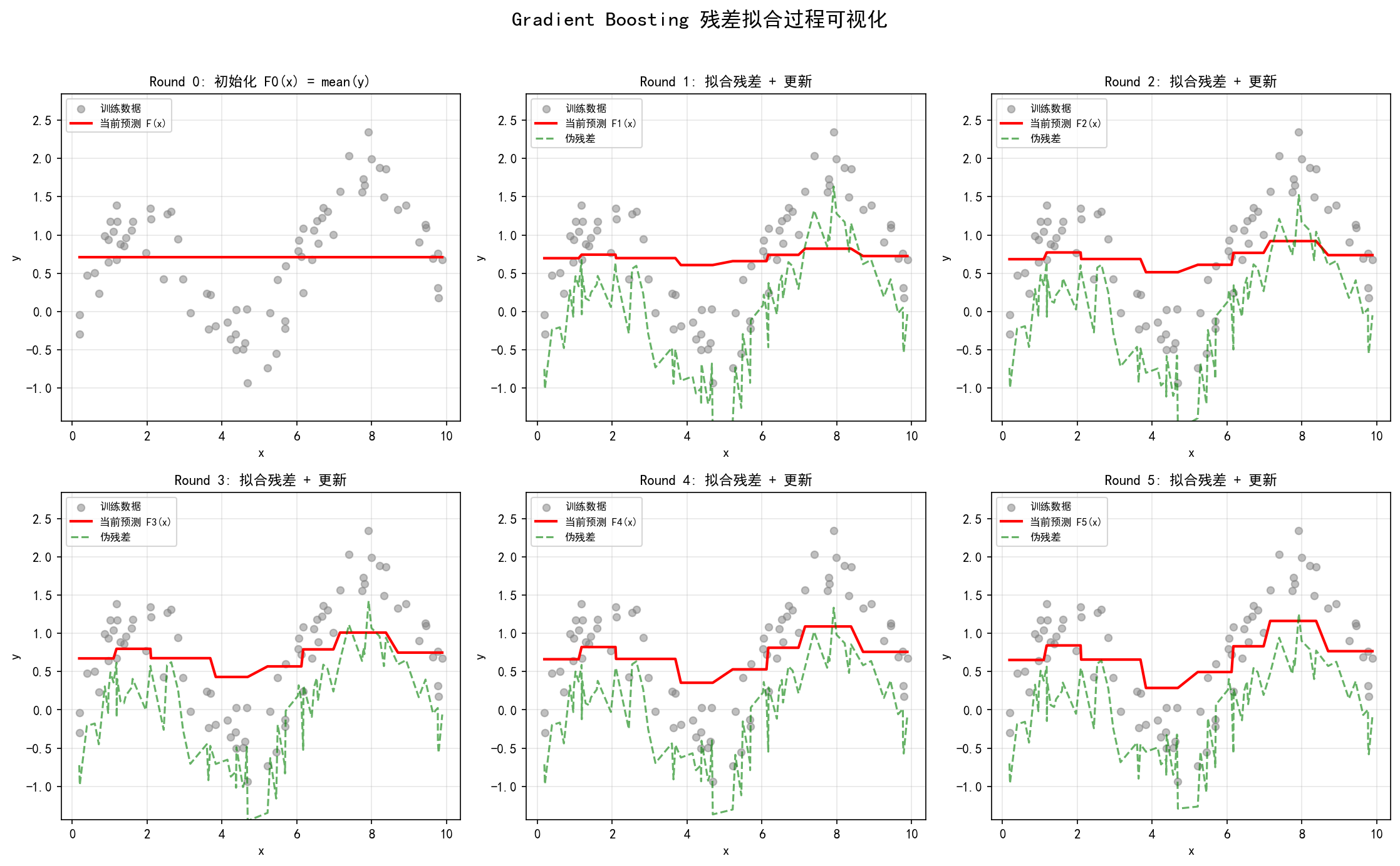
With squared-error loss, each new tree fits the current residuals. The learning rate scales its contribution to the ensemble.
5.1 Gradient descent in function space (Friedman 2001)
Jerome H. Friedman introduced gradient boosting in his 2001 paper “Greedy Function Approximation: A Gradient Boosting Machine” (released as a technical report in 1999). He recast boosting as gradient descent in function space, another major step in the theory of boosting that lifted AdaBoost from a specific algorithm to a general framework for function optimization.
Given training data $\{(x_i, y_i)\}_{i=1}^n$, the goal is to minimize a differentiable loss:
$$\mathcal{L}(F) = \sum_{i=1}^{n} L\big(y_i, F(x_i)\big)$$Notation: $F(x)$ is the mapping from inputs to predictions; $L(y, F)$ is the loss; $n$ is the number of training samples.
Ordinary gradient descent works in parameter space (the weights of a neural network, say). Gradient boosting makes $F(x)$ itself the object of optimization — gradient descent in function space. At iteration $m$, with current model $F_{m-1}(x)$, gradient descent says to move along the negative gradient of the loss with respect to the current prediction:
$$F_m(x) = F_{m-1}(x) - \rho_m \left. \frac{\partial L(y, F(x))}{\partial F(x)} \right|_{F=F_{m-1}}$$Notation: $\rho_m$ is the step size (set by line search); $\frac{\partial L}{\partial F}$ is the partial derivative of the loss with respect to the predicted value.
Strictly speaking, that expression is only defined at the training points $x_1, \ldots, x_n$: treat $\left(F(x_1), \ldots, F(x_n)\right)$ as an $n$-dimensional vector and the negative gradient is the $n$-dimensional vector $\left(r_{1m}, \ldots, r_{nm}\right)$ (see Section 5.2). Such a “gradient descent” only updates predictions at the training samples; it can’t be extended to new ones.
The key insight: $F$ is an arbitrary function and the negative gradient is only known at the training points, so we can’t work in the continuous function space directly. Friedman’s move was to use a weak learner (usually a shallow decision tree) $h_m(x)$ to approximate that negative gradient direction, turning function-space gradient descent into a computable sequence of models. Each new tree is trained to fit the current model’s “negative gradient,” and then its predictions enter the model weighted by the learning rate.
  graph TD
    A["Ordinary gradient descent
parameter space"] --> B["Update model parameters θ"]
    C["Gradient descent in function space
Friedman 2001"] --> D["Update the function F(x) itself"]
    D --> E["Use a weak learner h_m(x)
to approximate the negative gradient"]
    E --> F["Accumulate the update
old model plus new weak learner"]
5.2 Pseudo-residuals
Define the pseudo-residual of sample $i$ at iteration $m$ as
$$r_{im} = -\left[ \frac{\partial L(y_i, F(x_i))}{\partial F(x_i)} \right]_{F=F_{m-1}}$$Notation: $r_{im}$ is the pseudo-residual of sample $i$ at round $m$; $F_{m-1}(x_i)$ is the current model’s prediction for sample $i$.
Where the name comes from
- “Residual”: under squared loss $L(y, F) = \frac{1}{2}(y - F)^2$, the expression reduces to the ordinary residual $y_i - F_{m-1}(x_i)$, the difference between observed and predicted.
- “Pseudo”: under a general loss it is no longer that difference but the negative gradient of the loss with respect to the prediction. Only under squared loss does it coincide with the ordinary residual, hence the “pseudo.”
The pseudo-residual points in the direction that decreases the loss fastest at the current prediction. Each new weak learner is trained to fit these pseudo-residuals, which pushes the overall model toward lower loss. Geometrically, every gradient boosting step is a move in the steepest-descent direction on the tangent plane at the current function value.
  graph LR
    A["Current model"] --> B["Compute pseudo-residuals
negative gradient direction"]
    B --> C["Train weak learner h_m(x)
to fit the pseudo-residuals"]
    C --> D["Update the model
old model plus new weak learner"]
    D --> E["Loss decreases"]
5.3 The Taylor-expansion view (first-order gradient descent)
Gradient boosting can be seen as greedy optimization of a first-order Taylor expansion of the loss.
Let the current prediction be $F_{m-1}(x_i)$ and add a weak learner $h_m(x_i)$, so the new prediction is $F_{m-1}(x_i) + h_m(x_i)$. Expand the loss to first order around $F_{m-1}$:
$$L\big(y_i, F_{m-1}(x_i) + h_m(x_i)\big) \approx L\big(y_i, F_{m-1}(x_i)\big) + h_m(x_i) \cdot \left. \frac{\partial L}{\partial F} \right|_{F_{m-1}}$$Notation: $h_m(x_i)$ is the $m$-th weak learner’s prediction for sample $i$; $\frac{\partial L}{\partial F}$ is the partial derivative of the loss with respect to the current prediction.
Substituting the pseudo-residual:
$$L\big(y_i, F_{m-1}(x_i) + h_m(x_i)\big) \approx L\big(y_i, F_{m-1}(x_i)\big) - h_m(x_i) \cdot r_{im}$$To make the approximated loss drop, $\sum_i h_m(x_i)\, r_{im}$ should be as large as possible, which means $h_m$’s values on the training points should point the same way as the pseudo-residual vector. But the first-order approximation only holds for small $h_m$; chasing a larger inner product alone would drive the magnitude of $h_m$ to infinity. So gradient boosting splits the problem in two: first pick the direction — the function in the weak-learner class most “parallel” to the negative gradient, which Friedman (2001) does by least squares; then set the step size — how far to move, by line search (or per-leaf optimization, see Section 5.4):
$$h_m(x) = \arg\min_{h} \sum_{i=1}^{n} \big(r_{im} - h(x_i)\big)^2$$Notation: $h_m(x)$ is the optimal weak learner fitted to the pseudo-residuals; $r_{im}$ is the pseudo-residual of sample $i$ at round $m$.
This is exactly the core operation at each gradient boosting step: train a regression tree to fit the current model’s pseudo-residuals. Since a regression tree partitions the feature space into leaf regions and outputs a constant prediction in each, it offers a flexible and efficient way to approximate an arbitrary negative gradient direction.
5.4 A unified framework for any differentiable loss
One of Friedman’s (2001) central contributions was to extend boosting from AdaBoost’s exponential loss to a unified framework for any differentiable loss function. This is the fundamental reason gradient boosting is more general than AdaBoost.
| Task | Common loss | Pseudo-residual | Applications |
|---|---|---|---|
| Regression | Squared loss $\frac{1}{2}(y - F)^2$ | $y - F$ (ordinary residual) | General regression |
| Regression | Absolute loss $\lvert y - F \rvert$ | $\operatorname{sign}(y - F)$ | Regression with outliers |
| Regression | Huber loss | $y - F$ (when $\lvert y-F \rvert \leq \delta$); $\delta \operatorname{sign}(y-F)$ (otherwise) | Noise-robust regression |
| Regression | Quantile loss | $\tau - \mathbb{I}(y < F)$, i.e. $\tau$ when $y > F$ and $\tau - 1$ when $y < F$ | Prediction intervals, uncertainty estimation |
| Binary classification | Log loss, $y \in \{0,1\}$ | $y - \sigma(F)$ | Binary classification |
| Multiclass | Multinomial deviance | $y_{ik} - p_{k}(x_i)$ | $K$-class problems |
| Ranking | Pairwise ranking loss | Depends on the definition | Learning to rank |
The unified algorithm:
- Initialize: $F_0(x) = \arg\min_\gamma \sum_i L(y_i, \gamma)$
- For $m = 1, \dots, M$:
- Compute pseudo-residuals: $r_{im} = -\left[\frac{\partial L}{\partial F}\right]_{F_{m-1}}$
- Fit a weak learner: $h_m(x) = \arg\min_{h} \sum_i \big(r_{im} - h(x_i)\big)^2$
- Line search for the best step: $\rho_m = \arg\min_\rho \sum_i L\big(y_i, F_{m-1}(x_i) + \rho h_m(x_i)\big)$
- Update the model: $F_m(x) = F_{m-1}(x) + \nu \cdot \rho_m h_m(x)$
- Output: the final model $F_M(x)$
Notation: $\nu$ is the learning rate (shrinkage); $\rho_m$ is the optimal step from the line search; $M$ is the total number of iterations.
TreeBoost: line search per leaf. When the base learner is a regression tree with $J$ leaves, $h_m(x) = \sum_{j=1}^{J} b_{jm} \mathbb{I}(x \in R_{jm})$ is itself a combination of $J$ “basis functions.” Friedman (2001) recommends skipping a single global step $\rho_m$ and running the line search separately in each leaf region:
$$\gamma_{jm} = \arg\min_{\gamma} \sum_{x_i \in R_{jm}} L\left(y_i, F_{m-1}(x_i) + \gamma\right)$$then updating $F_m(x) = F_{m-1}(x) + \nu \sum_{j=1}^{J} \gamma_{jm} \mathbb{I}(x \in R_{jm})$. In other words, the tree only decides how to partition the regions, while each leaf’s output is re-optimized directly against the original loss. sklearn’s
GradientBoostingRegressor/Classifierand the pseudocode in Section 5.9 both take this form, and Sections 5.5 and 5.6 give the formula for $\gamma_{jm}$ under each loss.
  graph TD
    A["Choose a loss L"] --> B["Compute pseudo-residuals
r = -∂L/∂F"]
    B --> C["Train a regression tree on r"]
    C --> D["Line search for the best step ρ"]
    D --> E["Update F ← F + ν·ρ·h"]
    E --> F{"Converged?"}
    F -->|No| B
    F -->|Yes| G["Output F_M"]
5.5 The regression case (squared loss) in full
For regression, use the squared error (least squares) loss:
$$L(y, F) = \frac{1}{2}(y - F)^2$$Notation: $y$ is the true target; $F$ is the model prediction; the $\frac{1}{2}$ cancels the square when differentiating, which simplifies things.
Computing the pseudo-residual
$$r_{im} = -\frac{\partial}{\partial F}\left[\frac{1}{2}(y_i - F)^2\right]_{F=F_{m-1}} = -\left[-(y_i - F)\right]_{F=F_{m-1}} = y_i - F_{m-1}(x_i)$$The key result: under squared loss the pseudo-residual is exactly the ordinary residual (observed minus current prediction). So the intuitive reading of gradient boosting for regression is:
“Each new tree fits the residuals of the current ensemble, and its predictions join the ensemble weighted by the learning rate.”
The full regression procedure
Step 1: initialize
$$F_0(x) = \arg\min_\gamma \sum_{i=1}^{n} \frac{1}{2}(y_i - \gamma)^2 = \frac{1}{n}\sum_{i=1}^{n} y_i = \bar{y}$$Notation: $\bar{y}$ is the mean target over the training set; $\gamma$ is the constant prediction being optimized.
Under squared loss the best initial prediction is the training mean. That’s why many gradient boosting implementations initialize $F_0$ to mean(y).
Step 2: iterate ($m = 1, \dots, M$)
- Compute residuals: $r_{im} = y_i - F_{m-1}(x_i)$
- Fit a regression tree: $h_m(x)$ trained on $\{(x_i, r_{im})\}$, producing leaf regions $\{R_{jm}\}_{j=1}^{J_m}$
- For each leaf region $R_{jm}$, compute the optimal output:
Notation: $R_{jm}$ is the $j$-th leaf region of the $m$-th tree; $\lvert R_{jm} \rvert$ is the number of samples in it; $\gamma_{jm}$ is the optimal output for leaf $j$ (the mean residual in that leaf).
- Update the model:
Notation: $\nu$ is the learning rate (shrinkage); $\mathbb{I}(x \in R_{jm})$ is the indicator (1 when $x$ falls in leaf $R_{jm}$, otherwise 0).
Step 3: output $F_M(x)$
  graph TD
    subgraph "GB regression flow"
        A["Initialize to the target mean"] --> B["Compute current residuals"]
        B --> C["Train a regression tree on the residuals"]
        C --> D["Compute the optimal value γ_jm per leaf
mean residual in the leaf"]
        D --> E["Accumulate the leaf values into the model"]
        E --> F{"M rounds done?"}
        F -->|No| B
        F -->|Yes| G["Output F_M"]
    end
Other regression losses: LAD, Huber and quantile
Squared loss is sensitive to outliers. Friedman (2001) also gave TreeBoost algorithms for several robust losses; they differ in only three places: the initial value $F_0$, the pseudo-residual $r_{im}$ (see the table in Section 5.4) and the leaf value $\gamma_{jm}$.
| Loss | Initial $F_0$ | Leaf value $\gamma_{jm}$ |
|---|---|---|
| Squared loss (LS) | $\bar{y}$ | Mean of the in-leaf residuals $y_i - F_{m-1}(x_i)$ |
| Absolute loss (LAD) | $\operatorname{median}\{y_i\}$ | Median of the in-leaf residuals $y_i - F_{m-1}(x_i)$ |
| Quantile loss ($\tau$) | The $\tau$ quantile of $\{y_i\}$ | The $\tau$ quantile of the in-leaf residuals |
| Huber loss (M-TreeBoost) | $\operatorname{median}\{y_i\}$ | Median plus a one-step correction, see below |
The leaf values for LAD and quantile loss are exact: the $\gamma$ minimizing $\sum_{x_i \in R_{jm}} \lvert y_i - F_{m-1}(x_i) - \gamma \rvert$ is the median residual, and likewise for quantile loss. Note that here the tree is fitted to the pseudo-residual $\operatorname{sign}(y_i - F_{m-1}(x_i))$ (only $\pm 1$), while the leaf value is determined by the raw residuals — exactly TreeBoost’s “the tree sets the partition, the leaves are optimized separately.”
Huber loss has no closed-form leaf solution. Each round Friedman (2001) first sets the threshold $\delta_m$ to the $\alpha$ quantile of the current absolute residuals $\left\{\lvert y_i - F_{m-1}(x_i) \rvert\right\}$, then approximates the leaf value as “median plus one-step correction”: let $\tilde{r}_{jm}$ be the median of the residuals $r_{i} = y_i - F_{m-1}(x_i)$ within leaf $R_{jm}$ and $N_{jm}$ the number of samples there,
$$\gamma_{jm} = \tilde{r}_{jm} + \frac{1}{N_{jm}} \sum_{x_i \in R_{jm}} \operatorname{sign}\left(r_i - \tilde{r}_{jm}\right) \min\left(\delta_m, \lvert r_i - \tilde{r}_{jm} \rvert\right)$$In sklearn, loss='huber' and loss='quantile' share the alpha parameter: for the former it’s which quantile of the absolute residuals to use as $\delta_m$ (default 0.9), for the latter the quantile $\tau$ to estimate. Train one quantile model with alpha=0.05 and another with alpha=0.95 and you get a 90% prediction interval.
5.6 The classification case (log loss)
For binary classification, gradient boosting uses the log loss (binomial deviance):
$$L(y, F) = -y \log\big(\sigma(F)\big) - (1-y) \log\big(1 - \sigma(F)\big)$$Notation: $y \in \{0, 1\}$ is the class label; $\sigma(F) = \frac{1}{1 + e^{-F}}$ is the logistic sigmoid; $F(x)$ outputs log-odds, not a probability.
Computing the pseudo-residual
$$r_{im} = -\frac{\partial L}{\partial F}\bigg|_{F_{m-1}} = y_i - \sigma\big(F_{m-1}(x_i)\big) = y_i - p_i$$Notation: $p_i = \sigma(F_{m-1}(x_i))$ is the current model’s probability that sample $i$ is positive.
Key observations:
- Even for classification, each new tree is still a regression tree, because it fits a continuous gradient value (probability minus label) rather than a discrete class.
- The model output $F(x)$ is log-odds; the probability comes from $\sigma(F)$.
- When $y_i = 1$ and $p_i$ is near 0 (the model is wrong), the pseudo-residual is near 1 (the model should raise that sample’s log-odds sharply); when $p_i$ is near 1 (the model is right), it’s near 0 (no big adjustment needed).
- The pseudo-residual lies in $(-1, 1)$, so even badly misclassified samples exert bounded “pull” on the new tree. That’s one reason log loss is more robust than exponential loss.
Initial value and leaf values (Newton step)
Initial value: the optimal constant satisfies $\sum_i \left(y_i - \sigma(\gamma)\right) = 0$, i.e. $\sigma(\gamma) = \bar{y}$:
$$F_0(x) = \log\frac{\bar{y}}{1 - \bar{y}}$$that is, the log-odds of the positive-class rate $\bar{y}$ (which is exactly sklearn’s default initialization).
Leaf values: under log loss, $\gamma_{jm} = \arg\min_{\gamma} \sum_{x_i \in R_{jm}} L\left(y_i, F_{m-1}(x_i) + \gamma\right)$ has no closed form. Let $g_i$ and $h_i$ be the first and second derivatives of the loss with respect to $F$:
$$g_i = \frac{\partial L}{\partial F} = p_i - y_i, \qquad h_i = \frac{\partial^2 L}{\partial F^2} = p_i(1 - p_i)$$Starting from $\gamma = 0$, take one Newton-Raphson step:
$$\gamma_{jm} \approx -\frac{\sum_{x_i \in R_{jm}} g_i}{\sum_{x_i \in R_{jm}} h_i} = \frac{\sum_{x_i \in R_{jm}} (y_i - p_i)}{\sum_{x_i \in R_{jm}} p_i (1 - p_i)}$$This is how sklearn’s GradientBoostingClassifier computes leaf values (its source comments point to FHT 2000’s Newton step). Friedman’s original 2001 paper uses the $y \in \{-1, +1\}$ parameterization with $L = \log\left(1 + e^{-2yF}\right)$, where the pseudo-residual is $\tilde{y}_i = \frac{2y_i}{1 + e^{2y_i F_{m-1}(x_i)}}$ and the leaf value is $\gamma_{jm} = \frac{\sum \tilde{y}_i}{\sum \lvert \tilde{y}_i \rvert \left(2 - \lvert \tilde{y}_i \rvert\right)}$ — the same thing under a different parameterization.
Only one Newton step is taken here, rather than optimizing $\gamma$ to convergence in each leaf, as a compromise between cost and accuracy. XGBoost goes further and puts second-order information into the splitting criterion itself (Chapter 6).
The multiclass case ($K$ classes)
For a $K$-class problem you maintain one function $F_k(x)$ per class $k = 1, \dots, K$, using the multinomial deviance:
$$L\big(y, \{F_k\}\big) = -\sum_{k=1}^{K} \mathbb{I}(y = G_k) \log\big(p_k(x)\big)$$Notation: $G_k$ is the $k$-th class; $\mathbb{I}(y = G_k)$ is the indicator (1 when the sample’s true class is $G_k$, otherwise 0).
Class probabilities come from the softmax:
$$p_k(x) = \frac{\exp\big(F_k(x)\big)}{\sum_{l=1}^{K} \exp\big(F_l(x)\big)}$$Notation: $p_k(x)$ is the probability that sample $x$ belongs to class $k$; $F_k(x)$ is the score function (logit) for class $k$. Since softmax is invariant to adding the same function to all $F_k$, the $F_k$ are determined only up to a shared term; Friedman (2001) removes that degree of freedom with the constraint $\sum_{k=1}^K F_k(x) = 0$.
Pseudo-residual (for class $k$):
$$r_{ikm} = y_{ik} - p_{k, m-1}(x_i)$$Notation: $y_{ik} = \mathbb{I}(y_i = G_k)$ is the indicator label for class $k$; $p_{k, m-1}(x_i)$ is the current model’s probability for class $k$.
The multiclass procedure
- Initialize: $F_{k0}(x) = 0$ in Friedman’s (2001) original; sklearn initializes with the log of each class prior $\log \bar{y}_k$ (then subtracts the mean over classes so that $\sum_k F_{k0} = 0$), where $\bar{y}_k$ is the proportion of class $k$
- For $m = 1, \dots, M$:
- Compute probabilities from the current scores, $p_{k, m-1}(x_i)$ (softmax)
- For each class $k = 1, \dots, K$:
- Compute the pseudo-residual: $r_{ikm} = y_{ik} - p_{k, m-1}(x_i)$
- Fit a regression tree $h_{km}(x)$ to the pseudo-residuals
- Compute the optimal value for each leaf region (one Newton-Raphson step, Friedman 2001 Algorithm 6):
Notation: $R_{jkm}$ is the $j$-th leaf region for class $k$ at round $m$; $\gamma_{jkm}$ is that leaf’s optimal output. The factor $\frac{K-1}{K}$ comes from the constraint $\sum_k F_k = 0$.
- Update: $F_{km}(x) = F_{k, m-1}(x) + \nu \sum_{j} \gamma_{jkm} \, \mathbb{I}(x \in R_{jkm})$
- Output: $\hat{y} = \arg\max_k F_{kM}(x)$, with class probabilities $p_k(x) = \operatorname{softmax}\left(F_{1M}(x), \ldots, F_{KM}(x)\right)_k$
Note: each round fits $K$ trees, so multiclass gradient boosting takes roughly $K$ times as long to train as binary.
  graph TD
    subgraph "GB binary classification flow"
        A["Initialize F_0 = log(ȳ/(1-ȳ))
(log-odds of the positive rate)"] --> B["Compute pseudo-residuals r_i = y_i - p_i"]
        B --> C["Train a regression tree on r_i"]
        C --> D["Update the log-odds"]
        D --> E["Compute new probabilities p = σ(F_m)"]
        E --> F{"M rounds done?"}
        F -->|No| B
        F -->|Yes| G["Output sign(F_M)"]
    end
5.7 Regularization: shrinkage, subsampling, column sampling, tree complexity
Gradient boosting is greedy and prone to overfitting. In his 2001 and 2002 papers Friedman proposed several regularization strategies that underpin modern implementations such as XGBoost and LightGBM.
Shrinkage (learning rate)
The core update:
$$F_m(x) = F_{m-1}(x) + \nu \sum_{j=1}^{J_m} \gamma_{jm} \, \mathbb{I}(x \in R_{jm}), \quad 0 < \nu \leq 1$$Notation: $\nu$ is the learning rate (shrinkage factor), typically between $0.01$ and $0.3$; $\gamma_{jm}$ is the optimal value for each leaf of the $m$-th tree (Section 5.4).
How it works:
- With $\nu = 1$, each tree corrects the current error by the full (in-leaf) optimal step; training loss falls fast and the model overfits more readily.
- With $\nu < 1$, each tree contributes only part of the correction, spreading the learning over more rounds.
- A small $\nu$ makes learning more cautious: averaging many weak learners cancels the noise of individual trees and improves generalization noticeably.
Rule of thumb: learning rate and tree count trade off:
| learning_rate | Suggested n_estimators | When |
|---|---|---|
| 0.1 | 100-500 | Default; balances speed and quality |
| 0.05 | 500-2000 | Higher accuracy, tolerates slower training |
| 0.01 | 2000+ | Chasing the best performance, with early stopping |
Friedman (2001) found experimentally that a small learning rate ($\nu = 0.1$ or less) with enough trees markedly improves generalization. ESL §10.12.1 summarizes it: for a fixed number of rounds, smaller $\nu$ means higher training error, but empirically $\nu < 0.1$ usually gives better test error at the cost of a correspondingly larger $M$. So the usual practice is to set $\nu$ small and then choose $M$ with a validation set or early stopping.
Why shrinkage helps: in the limit of small steps under squared loss, “shrinkage + forward stagewise” traces a path resembling $L_1$ regularization (Lasso); ESL §16.2 discusses the connection between $\varepsilon$-forward stagewise and the Lasso, which supplies a regularization reading of shrinkage.
Subsampling (stochastic gradient boosting)
In “Stochastic Gradient Boosting,” Friedman (2002), inspired by Breiman’s bagging, proposed randomly drawing a subsample without replacement in each iteration to fit the current tree.
Changes to the algorithm:
- In each iteration $m$, draw a fraction $f$ (usually $f = 0.5$) of the training set as $S_m$
- Compute pseudo-residuals and fit $h_m$ using only $S_m$
- Updates still apply to predictions for all training samples
ESL §10.12.2 notes that a sampling fraction of $1/2$ is typical, and with large $N$ it can be well below $1/2$. In sklearn, setting subsample < 1.0 enables stochastic gradient boosting; samples not drawn in a round serve as out-of-bag (OOB) samples, and oob_improvement_ records each round’s loss improvement on them, a rough guide to a sensible number of iterations.
Regularization effect:
- Lower variance: different trees see different subsets, which increases diversity much as bagging does (sklearn’s docs note that
subsample < 1.0lowers variance and raises bias). - Less overfitting: the randomness stops the model from memorizing individual samples or outliers.
- Faster training: each tree fits a smaller dataset.
Column subsampling
Borrowing from random forests, consider only a random subset of features at each split (or per tree):
- Per split: sklearn’s
max_featuresis the number of features considered each time a best split is sought (XGBoost’scolsample_bynode). - Per tree / per level: XGBoost’s
colsample_bytree(once per tree) andcolsample_bylevel(once per level); LightGBM’sfeature_fraction(per tree).
Effect: less correlation between trees, lower variance, especially useful in high-dimensional feature spaces.
Controlling tree complexity
| Technique | Parameter | Typical range | Effect |
|---|---|---|---|
| Depth limit | max_depth | 3-6 | Caps each tree’s interaction order; depth=d captures at most d-way feature interactions |
| Minimum samples per leaf | min_samples_leaf | 5-50 | Stops leaves from overfitting single samples; smooths predictions |
| Minimum samples to split | min_samples_split | 2-20 | Controls when a node may split, avoiding overly fine splits |
| Maximum leaves | max_leaf_nodes | - | Controls tree size directly, an alternative to max_depth |
| Impurity decrease threshold | min_impurity_decrease | 0 | Pre-pruning: a split must earn enough gain |
Rules of thumb: a tree of depth 3 captures at most 3-way feature interactions; too much depth memorizes noise fast. More generally, a tree with $J$ leaves can represent feature interactions up to order $J-1$. ESL §10.11 reports that $4 \leq J \leq 8$ leaves usually works well in boosting and that results aren’t very sensitive to the exact value in that range; $J = 2$ (a stump) only yields an additive model with no interaction terms.
Summary of regularization techniques
| Technique | Parameter | Mechanism | Origin | Suggested |
|---|---|---|---|---|
| Shrinkage | learning_rate ($\nu$) | Scales each tree’s contribution | Friedman (2001) | 0.01-0.1, with more trees |
| Row subsampling | subsample | Trains each tree on a random subset | Friedman (2002) | 0.5-0.8 to lower variance |
| Column subsampling | max_features | Random feature subset per split | Random forest idea | sqrt or log2 |
| Depth limit | max_depth | Caps model complexity | General | 3-5 typical |
| Minimum leaf samples | min_samples_leaf | Smooths leaf predictions | General | 5-50 |
| Early stopping | n_iter_no_change | Stops when validation loss stalls | General | Stop after 10-20 rounds |
  graph TD
    A["Gradient boosting
overfits easily"] --> B["Shrinkage
learning_rate"]
    A --> C["Subsampling
subsample"]
    A --> D["Column sampling
max_features"]
    A --> E["Tree complexity control
max_depth/min_samples_leaf"]
    A --> F["Early stopping
n_iter_no_change"]
    B --> G["Reduce each tree's influence
spread out learning"]
    C --> H["More diversity between trees
bagging-style variance reduction"]
    D --> I["Less feature correlation
stops dominant features overfitting"]
    E --> J["Limit single-tree complexity
stops noise memorization"]
    F --> K["Avoid wasted iterations
save compute"]
    G --> L["Net effect:
better generalization"]
    H --> L
    I --> L
    J --> L
    K --> L
5.8 The sklearn API and key parameters
scikit-learn provides GradientBoostingClassifier and GradientBoostingRegressor, implementing the classic Gradient Boosting Machine.
GradientBoostingRegressor
| |
GradientBoostingClassifier
| |
Note: even for classification,
GradientBoostingClassifierfits regression trees internally (predicting gradient values) and gets probabilities through sigmoid or softmax at the end. Binary problems fit 1 tree per round; $K$-class problems fit $K$.Version note: for larger datasets (sklearn’s docs suggest
n_samples >= 10_000), scikit-learn recommends the histogram-basedHistGradientBoostingRegressor/Classifier, which is far faster (see Chapters 9 and 10).
Key parameters
| Parameter | Role | Suggested |
|---|---|---|
loss | Loss type | Use 'huber' for noisy data; 'quantile' when you need prediction intervals |
learning_rate | Scaling factor on each tree’s contribution | 0.01-0.1; smaller needs more trees |
n_estimators | Total number of trees | Tune together with learning_rate |
subsample | Fraction of samples per tree | 0.5-0.8 lowers variance |
max_depth | Tree depth | 3-5 typical; 3 is common for regression |
max_features | Feature sampling per split | 'sqrt' or 'log2' reduces overfitting |
min_samples_leaf | Minimum samples in a leaf | 5-50 guards against overfitting |
n_iter_no_change | Early-stopping patience | Setting 10 turns early stopping on |
Tuning advice
- Fix
learning_rate = 0.1first, and searchn_estimatorsandmax_depthwithGridSearchCVorRandomizedSearchCV. - Lower
learning_rate(to 0.05 or 0.01) while raisingn_estimators(500+), and use early stopping (n_iter_no_change). - Turn on subsampling: set
subsample=0.8or0.5; it usually works together with shrinkage. - Feature sampling: for high-dimensional data, try
max_features='sqrt'.
5.9 Pseudocode
Algorithm: Gradient Tree Boosting (regression)
- Input: training set $\{(x_i, y_i)\}_{i=1}^n$, loss $L(y, F)$, number of iterations $M$, learning rate $\nu$, tree depth $d$
- Output: the final model $F_M(x)$
- Initialize: $$F_0(x) \leftarrow \arg\min_\gamma \sum_i L(y_i, \gamma)$$ (for squared loss, $F_0(x) = \bar{y}$)
- For $m = 1, 2, \ldots, M$ do:
- Compute the pseudo-residuals: $$r_i \leftarrow -\left[\frac{\partial L(y_i, F(x_i))}{\partial F(x_i)}\right]_{F=F_{m-1}}, \quad i = 1,\ldots,n$$
- Fit a regression tree: $$h_m(x) \leftarrow \operatorname{TreeFit}\left(\{(x_i, r_i)\}_{i=1}^n;\ d\right)$$ i.e. fit a depth-$d$ regression tree to $\{(x_i, r_i)\}$ under squared error, producing leaf regions $\{R_{jm}\}_{j=1}^{J_m}$
- For each leaf $j = 1, \ldots, J_m$ do: $$\gamma_{jm} \leftarrow \arg\min_\gamma \sum_{x_i \in R_{jm}} L(y_i, F_{m-1}(x_i) + \gamma)$$ (for squared loss: $\gamma_{jm} = \frac{1}{\lvert R_{jm} \rvert}\sum_{x_i \in R_{jm}} r_i$, the mean in-leaf residual; for other losses see Sections 5.5 and 5.6)
- Update the model: $$F_m(x) \leftarrow F_{m-1}(x) + \nu \sum_{j=1}^{J_m} \gamma_{jm} \, \mathbb{I}(x \in R_{jm})$$
- Return $F_M(x)$
5.10 A from-scratch Python implementation (regression + classification, commented line by line)
| |
5.11 Cross-checking against sklearn
The code below systematically compares the custom implementations with sklearn’s GradientBoostingRegressor and GradientBoostingClassifier.
| |
5.12 Model interpretation: relative importance and partial dependence
Along with GBM, Friedman (2001) gave two tools for interpreting tree ensembles (ESL §10.13) that are still in wide use.
Relative importance: for a single tree $T$ with $J$ leaves ($J-1$ internal nodes), the importance of feature $X_\ell$ is defined as
$$\mathcal{I}_\ell^2(T) = \sum_{t=1}^{J-1} \hat{\imath}_t^2 \, \mathbb{I}\left(v(t) = \ell\right)$$where $v(t)$ is the splitting feature used at internal node $t$ and $\hat{\imath}_t^2$ is the squared-error reduction from that split. Averaging over $M$ trees gives the ensemble’s importance, $\mathcal{I}_\ell^2 = \frac{1}{M}\sum_{m=1}^{M} \mathcal{I}_\ell^2(T_m)$. sklearn’s feature_importances_ is this kind of impurity-decrease importance (normalized to sum to 1). Note that sklearn’s docs warn this measure favors high-cardinality features and is computed on the training set; when in doubt, compute permutation importance on a validation set with sklearn.inspection.permutation_importance.
Partial dependence: split the features into a subset of interest $X_S$ and the rest $X_C$, and define
$$\bar{f}_S(x_S) = \frac{1}{n} \sum_{i=1}^{n} F\left(x_S, x_{iC}\right)$$that is, replace every training sample’s $X_S$ with $x_S$, leave the other features alone, and average the model’s predictions. It describes how the model output moves with $x_S$ once the other features are averaged out. In sklearn, plot it with sklearn.inspection.PartialDependenceDisplay.from_estimator. When $X_S$ and $X_C$ are strongly correlated, this substitution produces feature combinations that don’t occur in reality, so read the result with care.
References
Core references for Chapter 4 (AdaBoost)
- Freund, Y. & Schapire, R. E. (1997). “A Decision-Theoretic Generalization of On-Line Learning and an Application to Boosting.” Journal of Computer and System Sciences, 55(1), 119-139.
- Freund, Y. & Schapire, R. E. (1996). “Experiments with a New Boosting Algorithm.” ICML.
- Friedman, J., Hastie, T. & Tibshirani, R. (2000). “Additive Logistic Regression: A Statistical View of Boosting.” The Annals of Statistics, 28(2), 337-407.
- Schapire, R. E., Freund, Y., Bartlett, P. & Lee, W. S. (1998). “Boosting the Margin: A New Explanation for the Effectiveness of Voting Methods.” The Annals of Statistics, 26(5), 1651-1686.
- Zhu, J., Zou, H., Rosset, S. & Hastie, T. (2009). “Multi-class AdaBoost.” Statistics and Its Interface, 2(3), 349-360. (2006 technical report version)
- Drucker, H. (1997). “Improving Regressors using Boosting Techniques.” ICML, 107-114.
- Wyner, A. J. (2003). “On Boosting and the Exponential Loss.” Proceedings of the Ninth International Workshop on Artificial Intelligence and Statistics (AISTATS 2003), 323-329.
- Schapire, R. E. & Singer, Y. (1999). “Improved Boosting Algorithms Using Confidence-rated Predictions.” Machine Learning, 37(3), 297-336.
- Breiman, L. (1999). “Prediction Games and Arcing Algorithms.” Neural Computation, 11(7), 1493-1517.
- Reyzin, L. & Schapire, R. E. (2006). “How Boosting the Margin Can Also Boost Classifier Complexity.” Proceedings of ICML 2006.
- Long, P. M. & Servedio, R. A. (2010). “Random Classification Noise Defeats All Convex Potential Boosters.” Machine Learning, 78(3), 287-304.
- Freund, Y. (2009). “A More Robust Boosting Algorithm.” arXiv:0905.2138.
- Schapire, R. E. (2013). “Explaining AdaBoost.” In Empirical Inference, Springer, 37-52.
- Li, H. (2019). Statistical Learning Methods (2nd ed.). Tsinghua University Press. Ch. 8.
Core references for Chapter 5 (Gradient Boosting)
- Friedman, J. H. (2001). “Greedy Function Approximation: A Gradient Boosting Machine.” The Annals of Statistics, 29(5), 1189-1232.
- Friedman, J. H. (2002). “Stochastic Gradient Boosting.” Computational Statistics & Data Analysis, 38(4), 367-378.
- Hastie, T., Tibshirani, R. & Friedman, J. (2009). The Elements of Statistical Learning (2nd ed.). Springer. Chapter 10.
- Bühlmann, P. & Hothorn, T. (2007). “Boosting Algorithms: Regularization, Prediction and Model Fitting.” Statistical Science, 22(4), 477-505.
- scikit-learn documentation: API reference for
GradientBoostingRegressor,GradientBoostingClassifier,AdaBoostClassifierandAdaBoostRegressor(version 1.9).
Generated: 2026-06-30. Role: classic algorithms writer.