
The boosting family is crowded — from classic AdaBoost to modern XGBoost, LightGBM and CatBoost — and each member has its own design philosophy, optimization target and sweet spot. On real projects, picking the right algorithm often matters more than fine-tuning it. This article compares the five mainstream boosting algorithms across several dimensions and lays out a practical decision procedure.
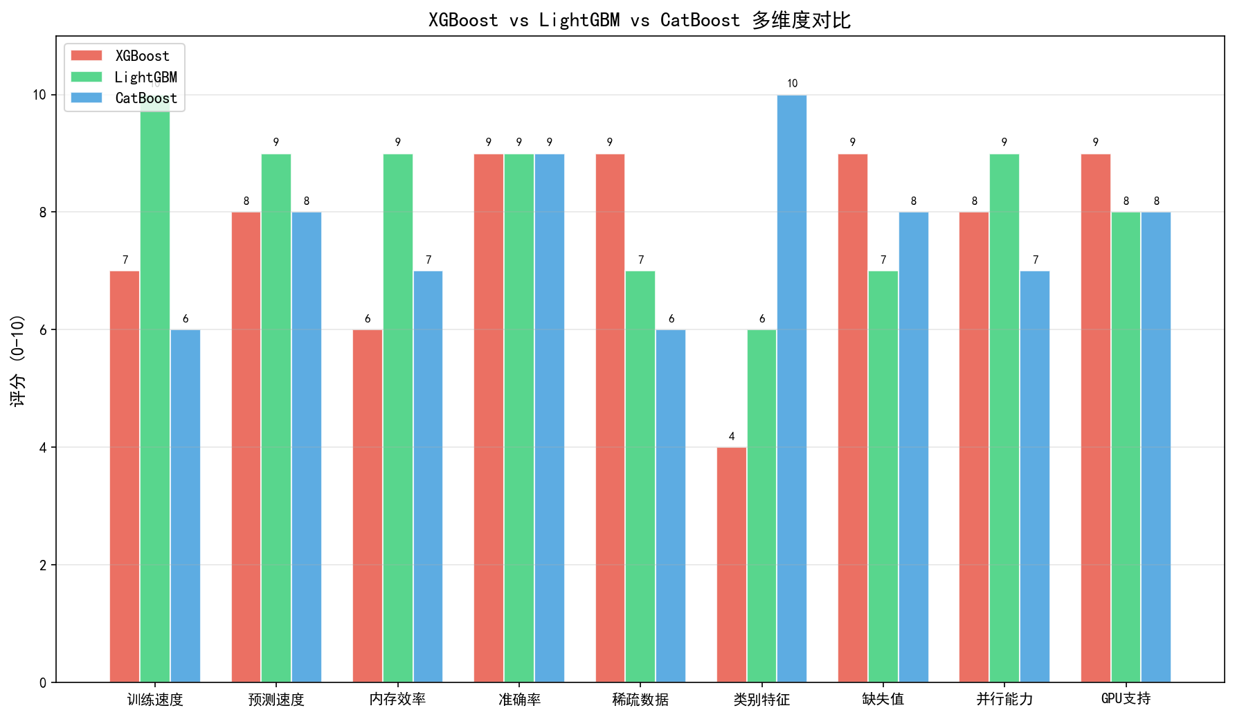
The comparison below covers training and prediction speed, memory use, accuracy, and feature handling.
9.1 The five algorithms side by side
The table compares AdaBoost, Gradient Boosting Machine (GBM), XGBoost, LightGBM and CatBoost across 11 dimensions: training speed, prediction speed, memory, accuracy, default-parameter behavior, sparse-data support, missing-value handling, categorical handling, GPU support, parallelism, and typical use cases.
| Dimension | AdaBoost (sklearn) | GBM (sklearn) | XGBoost | LightGBM | CatBoost |
|---|---|---|---|---|---|
| Core idea | Sample reweighting + exponential loss | Gradient descent in function space (first order) | Second-order Taylor expansion + explicit regularization | Histograms + leaf-wise growth + GOSS/EFB | Ordered boosting + oblivious trees |
| Training speed | ⭐⭐⭐ Slow (sequential, single-threaded, a full weak-learner fit per round) | ⭐⭐⭐ Slow (Cython, single-threaded, exact greedy splits, no histograms) | ⭐⭐⭐⭐ Fast (C++ core, multithreaded, hist histogram algorithm by default since 2.0) | ⭐⭐⭐⭐⭐ Usually fastest (histograms + leaf-wise growth + EFB; optional GOSS sampling) | ⭐⭐⭐⭐ Fast (symmetric trees; ordered target statistics for categoricals add cost, and explicit Ordered mode is slower) |
| Prediction speed | ⭐⭐⭐⭐⭐ Very fast (decision stumps need only a few comparisons) | ⭐⭐⭐⭐ Fast (shallow trees) | ⭐⭐⭐⭐ Fast (compact tree structure) | ⭐⭐⭐⭐ Fast (trees may be deeper but have few nodes) | ⭐⭐⭐⭐⭐ Very fast (symmetric trees compare once per level, which vectorizes well) |
| Memory | ⭐⭐⭐⭐⭐ Very low (the model is a handful of stumps) | ⭐⭐⭐⭐ Low (trains directly on raw float data) | ⭐⭐⭐⭐ Low (hist stores compressed bin indices; QuantileDMatrix saves more) | ⭐⭐⭐⭐⭐ Very low (bins stored as compact integers such as uint8) | ⭐⭐⭐⭐ Low (numeric features quantized into bins) |
| Out-of-the-box accuracy | ⭐⭐⭐ Middling (baseline level) | ⭐⭐⭐⭐ Good (the classic implementation) | ⭐⭐⭐⭐⭐ Excellent (regularization + second-order optimization) | ⭐⭐⭐⭐⭐ Excellent (leaf-wise fits more finely) | ⭐⭐⭐⭐⭐ Excellent (solid defaults, ordered target statistics reduce leakage) |
| Defaults | Reasonable (default n_estimators=50, learning_rate=1.0; tune those two plus base-learner depth) | Reasonable (max_depth=3, learning_rate=0.1; conservative) | Aggressive (max_depth=6, eta=0.3; needs tuning) | Aggressive (num_leaves=31, max_depth=-1 unlimited depth; pair with min_data_in_leaf) | Very friendly (almost no tuning; works out of the box) |
| Sparse data | ⭐⭐⭐ Fair (accepts scipy sparse matrices, but no special optimization) | ⭐⭐⭐ Fair (accepts scipy sparse matrices, but no special optimization) | ⭐⭐⭐⭐⭐ Excellent (sparsity-aware splits handle missing and zero values automatically) | ⭐⭐⭐⭐⭐ Excellent (histogram building skips zeros and the most frequent bin; EFB bundles exclusive sparse features) | ⭐⭐⭐⭐ Good (sparse input supported) |
| Missing values | Needs preprocessing (fit raises on NaN) | Needs preprocessing (fit raises on NaN) | ⭐⭐⭐⭐⭐ Learns the default direction for missing values | ⭐⭐⭐⭐⭐ Learns the default direction (use_missing=true) | ⭐⭐⭐⭐⭐ Numeric features treat missing as the minimum by default (nan_mode='Min') |
| Categorical features | Needs one-hot or similar | Needs one-hot or similar | ⭐⭐⭐⭐ Native since 1.5 (enable_categorical=True, pandas category columns) | ⭐⭐⭐⭐ Native (non-negative integers or pandas category; partitions after sorting by gradient statistics) | ⭐⭐⭐⭐⭐ Native (ordered target statistics + feature combinations) |
| GPU | ❌ None | ❌ None | ✅ Yes (since 2.0 via device='cuda'; the old gpu_hist is deprecated) | ✅ Yes (device_type='gpu' for OpenCL, 'cuda' for CUDA, with the matching build) | ✅ Yes (task_type='GPU', multi-GPU supported) |
| Parallelism | ⭐⭐ Weak (no n_jobs; weak learners train sequentially) | ⭐⭐ Weak (no n_jobs; single-threaded) | ⭐⭐⭐⭐ Strong (OpenMP threads; distributed training via Dask, Spark and others) | ⭐⭐⭐⭐⭐ Very strong (feature, data and voting parallelism) | ⭐⭐⭐⭐ Strong (CPU threads via thread_count, multiple GPUs) |
| Typical use | Quick baselines, small binary classification, teaching | Small to medium data, sklearn ecosystem integration | Competition workhorse, large tabular data, custom objectives | Very large data, high-dimensional features, memory-constrained settings | Data with many categorical features, plug-and-play needs, robust defaults on small data |
On sklearn’s
HistGradientBoosting: “GBM (sklearn)” above means the classicGradientBoostingClassifier/GradientBoostingRegressor. scikit-learn also shipsHistGradientBoostingClassifier/HistGradientBoostingRegressor, inspired by LightGBM (introduced as experimental in 0.21, stable from 1.0): it uses histograms and OpenMP threads, natively handles missing values (learning where they go) and categorical features (defaultcategorical_features='from_dtype'since 1.6, detecting pandas/polars category columns), and supports monotonic and interaction constraints plus built-in early stopping. The docs recommend it over classic GBM once you have tens of thousands of samples.
Reading the key differences
1. Where the training-speed differences come from
AdaBoost and sklearn’s classic GBM use sklearn decision trees as base learners with exact greedy splitting: at each node they sort each feature’s values and scan candidate split points, so a node costs roughly $O(nd\log n)$ with $n$ samples and $d$ features. XGBoost and LightGBM’s histogram methods discretize continuous features into $b$ buckets: building the histogram is about $O(nd)$, and searching splits over buckets about $O(db)$. Since $b$ is usually far smaller than $n$, sorting and candidate scanning get much cheaper. LightGBM additionally uses leaf-wise growth and EFB (exclusive feature bundling) and can enable GOSS (gradient-based one-side sampling; off by default, turned on in 4.x with data_sample_strategy='goss'), which usually makes it faster on large data. On CPU, CatBoost defaults to boosting_type='Plain' (the classic gradient boosting scheme, still with ordered target statistics for categoricals); ordered boosting is used only when you set boosting_type='Ordered', or on GPU with at most 50,000 samples and a non-multiclass task. Target statistics and feature combinations add cost, and Ordered mode is slower, so CatBoost is usually a little behind LightGBM on raw speed but clearly ahead of classic GBM.
2. Where the memory differences come from
LightGBM’s histogram method discretizes continuous features into at most 255 buckets by default (max_bin=255), so each value costs one uint8 bin index — about $1/8$ of the raw float64 data. XGBoost’s default hist tree method likewise stores only compressed bin indices (default max_bin=256), and QuantileDMatrix can skip keeping an intermediate copy of the raw data; only the old exact method’s pre-sorted blocks needed raw float values. CatBoost also quantizes numeric features into bins first (CPU default border_count=254). AdaBoost’s stumps store just one threshold and one feature index, so the model itself takes almost no memory, though training still has to sort the raw float data.
3. Default accuracy and parameter sensitivity
CatBoost is known for working out of the box: its defaults already perform well on many datasets, and the learning rate is chosen from data size and iteration count (see Chapter 10). XGBoost and LightGBM default to more aggressive settings (XGBoost’s max_depth=6, eta=0.3), which overfit readily on small and medium data and call for tuning. AdaBoost’s default stumps (max_depth=1) usually underfit; you need deeper trees or more rounds to unlock it. sklearn GBM’s max_depth=3 is relatively conservative and a decent starting point.
4. Missing values and sparse data
XGBoost’s sparsity-aware split finding is its signature innovation: at each split the algorithm learns whether missing values should go left or right, by enumerating both directions and taking the larger gain. The mechanism handles not just missing values but the zeros from one-hot encoding and plain statistical sparsity. LightGBM skips zeros (and the most frequent bin) while building histograms, and handles missing values much as XGBoost does: use_missing=true by default, trying missing-on-the-left and missing-on-the-right at each split and keeping the better direction; zero_as_missing=true also treats zeros as missing. CatBoost defaults to nan_mode='Min' for numeric features, treating missing as smaller than every value and ensuring “missing vs. everything else” is among the candidate splits; for categorical features it does nothing special — a missing value is just another category. Classic AdaBoost and sklearn GBM, by contrast, need missing values filled in during preprocessing (mean, median or a sentinel), or training fails (sklearn’s HistGradientBoosting and, since 1.4, random forests do accept NaN).
5. Native categorical support
All three modern libraries handle categoricals natively, but differently. CatBoost converts them into numeric ordered target statistics: each sample’s statistic uses only the labels of samples preceding it in a random permutation, which avoids the target leakage of conventional target encoding, and it also builds categorical combinations automatically. LightGBM requires non-negative integers or pandas category (category columns detected automatically; numpy input must be declared via categorical_feature), and finds the best partition by sorting categories by their gradient statistics. XGBoost has supported categoricals under hist/approx since 1.5 (enable_categorical=True with pandas category columns), and partition-based splits since 1.6. Classic AdaBoost and sklearn GBM require you to encode categoricals before training (one-hot or ordinal); one-hot on high-cardinality features creates a flood of sparse columns that hurts split efficiency.
9.2 A decision tree for choosing an algorithm
How do you pick quickly on a specific project? The flowchart below gives a systematic path.
  flowchart TD
    A["Start: look at the dataset"] --> B{"Data size?"}
    B -->|small, low-dimensional| C{"Many categorical features?"}
    B -->|large or high-dimensional| D{"Is training speed critical?"}

    C -->|Yes| E["Prefer CatBoost
native categorical support
works out of the box"]
    C -->|No| F{"Need a quick baseline?"}
    F -->|Yes| G["AdaBoost
stumps train fast
good for understanding the theory"]
    F -->|No| H["sklearn HistGradientBoosting / GBM
no extra dependencies
seamless with the sklearn ecosystem"]

    D -->|Yes| I{"Memory constrained?"}
    D -->|No| J{"Many categorical features?"}

    I -->|Yes| K["LightGBM
histograms, low memory
leaf-wise, fast training"]
    I -->|No| L["XGBoost or LightGBM
both are fast"]

    J -->|Yes| E
    J -->|No| M{"Need GPU acceleration?"}
    M -->|Yes| N["XGBoost or CatBoost
mature GPU support
LightGBM needs a GPU build"]
    M -->|No| O{"Need interpretability or custom objectives?"}
    O -->|Yes| P["XGBoost
custom objectives
solid SHAP support"]
    O -->|No| Q{"Chasing speed or accuracy?"}
    Q -->|speed| K
    Q -->|accuracy| R["XGBoost or CatBoost
competition-grade accuracy"]
The decision points
Node B: how big is the data?
Data size is the first consideration. On small datasets (under 10,000 samples, under 50 features) training time barely differs between algorithms, so accuracy and ease of use should decide. CatBoost’s defaults are usually robust on small data and need no categorical preprocessing; with few samples you can also explicitly try boosting_type='Ordered'. On large datasets training speed and memory become the bottleneck, so a modern efficient implementation (XGBoost, LightGBM, CatBoost) is required.
Node D: is training speed critical?
If the model is retrained frequently — a recommender updated daily, a real-time risk model — training speed matters. LightGBM is usually the fastest choice, especially on high-dimensional data. If training happens once (an annual churn model, say), you can trade speed for accuracy.
Node I: memory-constrained settings
On edge devices, embedded systems, or individual workers in a large distributed cluster, memory may be tight. LightGBM’s histogram method compresses feature values into 8-bit bin indices, so memory use is low (XGBoost’s hist uses similar compressed storage). If memory is extremely tight — a few hundred MB — you could even consider AdaBoost (stumps take almost no memory), at the cost of accuracy.
Node J: how many categorical features?
With many categorical features (user IDs, product categories, geographic codes), CatBoost is the first choice. Its Ordered TS encoding removes manual preprocessing and usually beats one-hot on high-cardinality features. A feature with 1,000 categories, for instance, becomes 1,000 binary columns under one-hot, which makes splits inefficient, whereas CatBoost uses the original categorical column directly. (CatBoost only one-hot encodes features with at most one_hot_max_size categories, generally 2 by default on CPU.) LightGBM’s and XGBoost’s native categorical support also avoids one-hot blowup, but they overfit more readily at high cardinality and need parameters such as cat_smooth and max_cat_threshold.
Node O: custom objectives
XGBoost has the most flexible custom-objective interface: define the first derivative $g_i$ and the second derivative $h_i$ and you’re done. That’s valuable when optimizing a non-standard business metric (Focal Loss for class imbalance, Huber loss for regression outliers, a custom ranking loss). LightGBM (a callable objective in the sklearn interface; a callable in params['objective'] since 4.0 in the native one) and CatBoost (a Python class implementing calc_ders_range) support custom objectives too, but XGBoost has by far the richest tutorials and community examples.
9.3 When each algorithm fits
AdaBoost
AdaBoost works best as a teaching tool and a quick baseline. Its logic is clean, and each round visibly demonstrates “focus on misclassified samples,” which makes it excellent for explaining the ideas. It still earns its place in a few situations:
- Very small binary problems (under 1,000 samples) with low-dimensional features (under 20)
- Fast data sanity checks: run the whole pipeline end to end with default AdaBoost and confirm the data loads and labels are right
- A first pass at feature importance:
feature_importances_weights each base learner’s impurity importance by its weight, which quickly surfaces the more important features; but impurity-based importance favors high-cardinality features, so pair it with permutation importance for serious analysis (see Section 11.5) - Reproducing textbook experiments: when you need to replicate algorithm experiments from ESL or a textbook, sklearn’s AdaBoost is the most direct implementation
Its limits: exponential loss is sensitive to mislabeled samples and outliers (they get reweighted repeatedly), rounds can’t be parallelized, there’s no native support for missing values or categoricals, and on most tasks its accuracy trails modern gradient boosting. In most production settings, gradient boosting has replaced it.
sklearn GBM
sklearn’s GradientBoostingClassifier/GradientBoostingRegressor is a faithful implementation of classic gradient boosting, suited to:
- Deep integration with the sklearn ecosystem: using
Pipeline,GridSearchCV,cross_val_scoreand so on without pulling in external dependencies (XGBoost, LightGBM and CatBoost are all third-party) - Fully understanding GBM internals: sklearn’s Python/Cython code reads more easily than XGBoost’s C++ core, which suits source study and algorithm research
- Small to medium data (under 100,000 samples) where training speed isn’t critical
- Specific losses:
Huber Loss(robust regression),Quantile Loss(quantile prediction) — sklearn GBM supports these natively with a stable API
Its main drawbacks are slower training (exact greedy splits, single-threaded, no GPU) and no missing-value support. (The old presort parameter was deprecated in 0.22 and removed in 0.24.) HistGradientBoostingClassifier/HistGradientBoostingRegressor, experimental in 0.21 and stable from 1.0, are histogram-based and support threading, missing values and categorical features, which makes them considerably faster; they’re the preferred in-sklearn replacement. They also cover the Huber and quantile losses listed above (loss='quantile'; Huber still needs classic GBM).
XGBoost
XGBoost is the evergreen of tabular competitions and fits almost any structured-data task:
- Competitions and benchmarks: on Kaggle, Tianchi and the like, XGBoost is usually the first algorithm tried and a core component of the final ensemble
- Large data (millions of samples): histogram approximation, block structure and out-of-core computation let it handle data larger than memory
- Custom objectives and metrics: a custom ranking loss for credit risk, a weighted log loss for medical prediction
- Interpretability: XGBoost ships TreeSHAP (
predict(..., pred_contribs=True), orpred_interactions=Truefor interaction values) and works with the SHAP library for global importance, individual explanations and dependence plots (LightGBM’spred_contrib=Trueand CatBoost’sget_feature_importance(type='ShapValues')offer similar capabilities) - Data with many missing values: sparsity-aware splits learn the best direction, with no need to guess an imputation strategy
- Distributed training: XGBoost supports Dask, Spark and Ray, which suits enterprise big-data platforms
XGBoost 2.0 brought several improvements: a unified device parameter (device='cuda' for GPU, retiring gpu_hist), hist as the default tree method, experimental multi-output trees (multi_strategy='multi_output_tree'), a quantile regression objective (reg:quantileerror), and a rewritten learning-to-rank implementation.
LightGBM
LightGBM is the first choice for large data and high-dimensional features, especially for:
- Very large data (tens of millions of samples and up): histograms, leaf-wise growth and EFB usually make training fast, and
data_sample_strategy='goss'enables GOSS sampling for more speed (how much faster than XGBoost’shistdepends on the data — measure it) - High-dimensional sparse features (user-item cross features or text features in CTR prediction): EFB bundles exclusive sparse features and cuts the effective feature count sharply
- Severely constrained memory: limited Kaggle Notebook memory, edge deployment
- Real-time training: minute-scale model refreshes in online advertising
- Categoricals already label-encoded: less elegant than CatBoost’s native support, but fine once declared via
categorical_feature
Leaf-wise growth lets LightGBM build deeper trees than XGBoost’s level-wise strategy at the same num_leaves, which fits better and overfits more easily. The official tuning docs therefore name num_leaves as the primary complexity control, recommend pairing it with min_data_in_leaf, and suggest max_depth as a last resort. LightGBM 4.0 removed the early_stopping_rounds argument from train(), cv() and the sklearn fit() (use the lgb.early_stopping() callback instead), added data_sample_strategy, and gave the Linux manylinux wheel built-in OpenCL GPU support (just pass device='gpu' after pip install lightgbm).
CatBoost
CatBoost stands apart for working out of the box and for categorical handling, which suits:
- Data with many categorical features: e-commerce (user ID, product ID, brand, category), finance (transaction type, merchant category code), healthcare (ICD diagnosis codes)
- Plug and play, little tuning time: when deadlines are tight and there’s no room for extensive grid search, CatBoost’s defaults are often competitive already
- Reducing target-leakage risk: ordered target statistics avoid the leakage of target encoding, and ordered boosting further mitigates prediction shift in gradient estimation — though it isn’t on by default on CPU (the default is
boosting_type='Plain'); tryboosting_type='Ordered'on small datasets - Well-structured trees: oblivious trees share one split condition across a level, giving them a regular structure, a strong regularizing effect, and fast predictions
- Fast deployment: CatBoost’s compact model format and high-performance C++ inference library suit low-latency production deployment
Beyond categoricals, CatBoost natively supports text features (text_features) and embedding features (embedding_features) and offers grid_search/randomized_search for simple hyperparameter search. When categorical features — especially high-cardinality ones — dominate the data, CatBoost is usually worth trying first.
9.4 Recent version changes
As of November 2026, the versions used to test this book’s code are scikit-learn 1.9.1, XGBoost 3.4.1, LightGBM 4.7.0 and CatBoost 1.2.10. The table lists the changes in recent major versions that most affect practice (defer to each library’s official changelog).
| Library | Version | Key changes | Practical impact |
|---|---|---|---|
| scikit-learn | 1.0 / 1.4 / 1.6 / 1.8 | 1.0: HistGradientBoosting stable; 1.4: AdaBoostClassifier’s algorithm='SAMME.R' deprecated, HistGradientBoosting gains categorical_features='from_dtype'; 1.6: SAMME.R removed, the algorithm parameter deprecated, 'from_dtype' becomes the default; 1.8: algorithm removed | Don’t pass algorithm to AdaBoostClassifier in new code; prefer HistGradientBoosting as the fast replacement for classic GBM |
| XGBoost | 2.0 / 3.x | 2.0: device unifies CPU/GPU (gpu_hist deprecated), hist becomes the default tree method, experimental multi-output trees via multi_strategy, reg:quantileerror; early_stopping_rounds moves from fit() to the constructor (deprecated in 1.6, old form removed in 2.1); 3.0: the old binary model format can no longer be saved (and can’t be loaded from 3.1) | Train on GPU with device='cuda'; save models as .json or .ubj (see Section 11.4) |
| LightGBM | 4.0 / 4.x | 4.0: removes old parameters such as early_stopping_rounds and verbose_eval (callbacks instead), adds data_sample_strategy (GOSS becomes data_sample_strategy='goss'), rewrites the CUDA version (device_type='cuda'), adds built-in OpenCL GPU support to the Linux wheel; 4.7: sklearn fit() gains eval_X/eval_y and deprecates eval_set | Use the lgb.early_stopping() callback for early stopping; don’t write boosting='goss' for GOSS |
| CatBoost | 1.2.x | The 1.2 series keeps improving GPU training and compatibility with new Python/NumPy releases; boosting_type defaults to 'Plain' on CPU, and non-multiclass CPU tasks default to bootstrap_type='MVS' (bagging_temperature only applies under 'Bayesian') | On small datasets try boosting_type='Ordered' explicitly; control sampling strength with subsample, not bagging_temperature |
Version guidance
- New projects: use XGBoost 2.0+ or LightGBM 4.0+, both mature in speed, features and stability. If the data has many categorical features, choose CatBoost 1.2+.
- Maintaining old projects: before upgrading to sklearn 1.8+, delete
AdaBoostClassifier(algorithm=...)or it raisesTypeError; when upgrading XGBoost/LightGBM, check for oldfit()arguments such asearly_stopping_rounds. Consider migratingGradientBoostingtoHistGradientBoostingfor the speedup. - Production: all three offer C/C++ inference interfaces and export paths such as ONNX, with XGBoost and LightGBM having the richest deployment docs and community material; CatBoost’s symmetric trees predict fast, which suits latency-sensitive settings such as real-time recommendation.
- Research: if you’re working on algorithm variants or custom losses, XGBoost’s interface flexibility and extensibility are the best of the three.
9.5 Boosting versus random forests and deep learning
The comparisons so far stay inside the boosting family. Real projects also raise the question: should this be a random forest, or a neural network?
Versus random forests (bagging): a random forest trains deep trees independently in parallel and mainly reduces variance; boosting fits residuals (negative gradients) in sequence and mainly reduces bias (see Chapter 1). Random forests are insensitive to hyperparameters, practically never overfit from having too many trees, parallelize naturally, and make dependable baselines; well-tuned gradient boosting is more accurate on most tabular tasks but is more sensitive to learning rate, tree count and tree complexity, and needs early stopping. When the training set is small, the noise is heavy, or there’s no time to tune, a random forest is often the easier choice.
Versus deep learning: on typical tabular data of moderate size (roughly ten thousand to tens of thousands of samples), several benchmark studies find that tuned tree ensembles (XGBoost, random forests) still beat deep models designed specifically for tabular data, at far lower training cost. Grinsztajn et al. (NeurIPS 2022) put it down to three things: neural networks favor overly smooth solutions and struggle with irregular functions; they’re less robust to uninformative features; and they’re rotation-invariant, whereas tabular features each carry meaning. Shwartz-Ziv and Armon (2022) also found XGBoost beating several deep tabular models on most datasets, with ensembles of the two usually best. Deep learning’s edge is unstructured data — images, text, audio — and settings that need end-to-end representation learning, multimodal fusion, or continuous training on very large data.
| Situation | What to do |
|---|---|
| Structured tabular data, up to a million rows | Try LightGBM / XGBoost / CatBoost first, with a random forest as baseline |
| Almost no time to tune, or very small and noisy data | Random forest, or CatBoost with defaults |
| Images, text, speech and other unstructured data | Deep learning (network embeddings can be fed to a GBDT as features) |
| Tabular data mixed with long text or image fields | Extract embeddings with a pretrained model and feed them to a GBDT alongside tabular features; or train a multimodal network |
| Competition-grade accuracy | Ensemble several GBDTs and neural networks (stacking / weighted averaging; see Chapter 1) |