
Hyperspectral remote sensing is a key technique for identifying the endmember constituents within a target region and their proportions. It is widely used in land-cover classification, environmental monitoring, and related fields. Hyperspectral unmixing (HU) is the signal-processing task of analyzing hyperspectral data to identify the endmembers in an image and their corresponding abundances. Craig’s minimum-volume simplex criterion is a classical and effective method for blind unmixing: the vertices of the minimum-volume simplex that encloses the data point cloud are taken as the endmember estimates. Related algorithms are computationally inefficient, however, because they involve complicated volume calculations. HyperCSI (Hyperplane-based Craig-Simplex Identification) does not evaluate a complicated volume function. It uses a geometric theorem instead: an \(N\)-dimensional simplex can be determined by \(N\) hyperplanes (of dimension \(N-2\)). HyperCSI reconstructs Craig’s minimum-volume simplex by constructing \(N\) hyperplanes associated with it. This avoids the volume calculation and is far less expensive than algorithms based on Craig’s criterion.
Principle of the Algorithm
1. Assumptions and Notation
Let the observed data be \(\{x[1],\dots,x[L]\} \subset \mathbb{R}^M\), where each \(x[n] \in \mathbb{R}^M\) is a pixel vector in the image and contains the values of \(M\) spectral bands. The vector \(x[n]\) is assumed to be a linear combination of \(N\) endmembers \(\{a_1,\dots,a_N\}\subset \mathbb{R}^M\), and the abundance vector \(s[n] = [s_1[n],\dots,s_N[n]]^T \in \mathbb{R}^N\) satisfies the nonnegativity constraint and sums to one. That is,
\[ x[n] = \sum_{i=1}^N s_i[n] a_i + w[n], \quad \forall n \in \{1,\dots,L\} \]where \(w[n]\) is additive noise. Let \(\alpha_i = C^\dagger (a_i-d) \in \mathbb{R}^{N-1}\) be the endmember vector after dimension reduction (DR), where \(C\in\mathbb{R}^{M \times (N-1)}\) is the matrix whose columns are the eigenvectors corresponding to the first \(N-1\) principal components of the data matrix, and \(d=\frac{1}{L}\sum_{n=1}^L x[n]\) is the data mean. The data after DR are then
\[ \tilde{x}[n] = C^\dagger (x[n] - d) = \sum_{i=1}^N s_i[n]\alpha_i \in \mathbb{R}^{N-1} \]2. Representing Craig’s Minimum-Volume Simplex by Hyperplanes
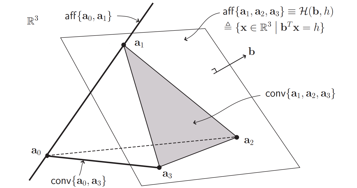
Let Craig’s minimum-volume simplex be \(\mathcal{T} = \mathrm{conv}\{\alpha_1,\dots,\alpha_N\} \subset \mathbb{R}^{N-1}\). By the following proposition, this simplex can be determined by \(N\) associated hyperplanes \(H_1,\dots,H_N\):
Proposition 1. If \(\{\alpha_1,\dots,\alpha_N\}\subset\mathbb{R}^{N-1}\) are affinely independent (that is, \(\mathcal{T}\) is a simplex), then \(\mathcal{T}\) can be reconstructed from \(N\) hyperplanes \(\{H_1,\dots,H_N\}\) that tightly enclose \(\mathcal{T}\), where \(H_i = \text{aff}(\{\alpha_1,\dots,\alpha_N\}\backslash\{\alpha_i\})\).
Proof sketch: it is enough to show that \(\{\alpha_1,\dots,\alpha_N\}\) can be determined from \(\{H_1,\dots,H_N\}\). The proof is omitted.
The key step of HyperCSI is therefore to estimate these \(N\) hyperplanes, recover Craig’s minimum-volume simplex, and thereby obtain the endmember estimates.
3. Estimating Hyperplane Normals
Now consider how to estimate the normal \(b_i\) and the constant \(h_i\) of the \(i\)-th hyperplane \(H_i(b_i,h_i) = \{x\in\mathbb{R}^{N-1} \ \vert \ b_i^T x = h_i\}\).
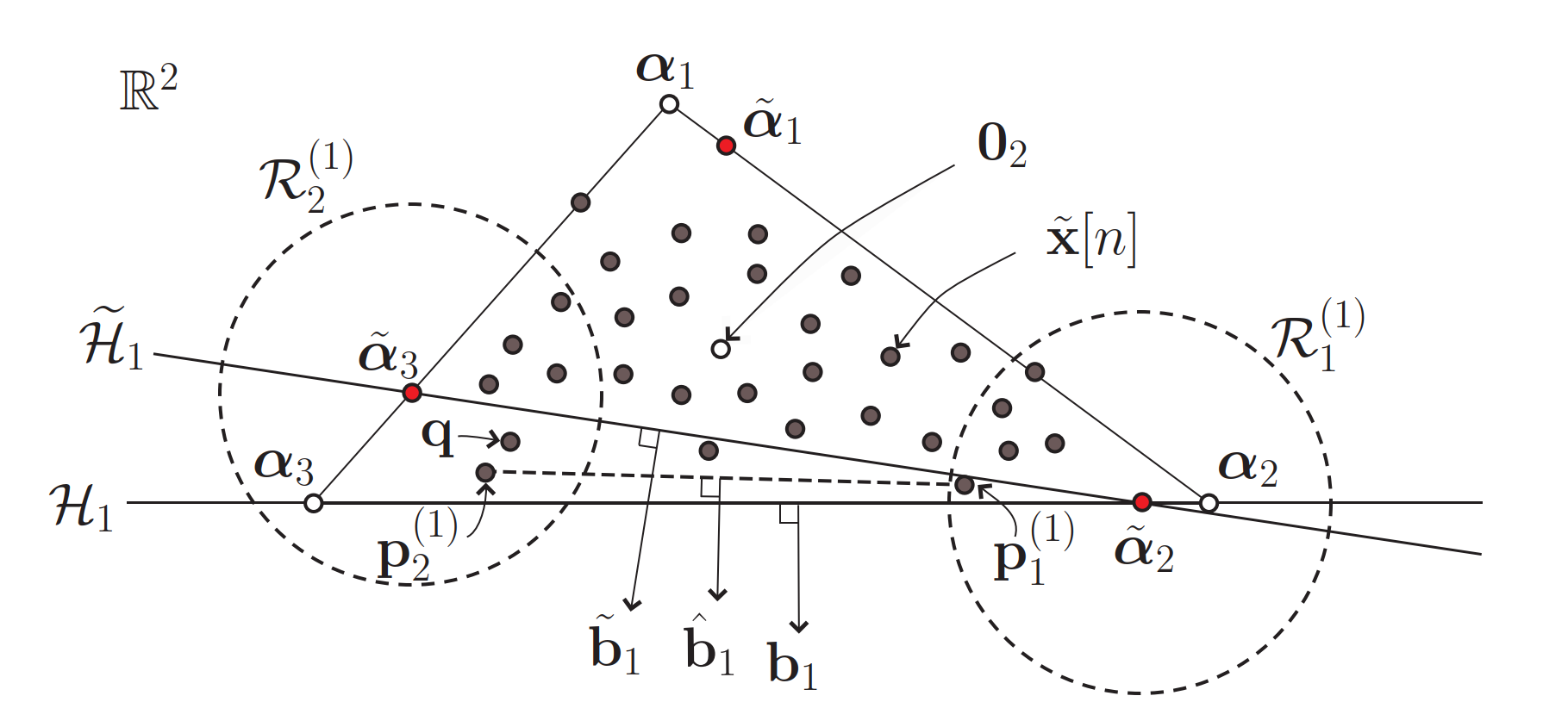
By the following proposition, \(b_i\) is determined once any \(N-1\) affinely independent points on \(H_i\) have been found.
Proposition 2. Given any set of \(N-1\) affinely independent points \(\{p_1^{(i)},\dots,p_{N-1}^{(i)}\}\subset H_i\) on \(H_i\), one has (up to a positive scale factor)
\[ b_i = v_i (p_1^{(i)}, \dots, p_{N-1}^{(i)}) \]where
\[ v_i(p_1, \dots, p_{N-1}) = (I_{N-1} - P(P^TP)^{-1}P^T)(p_j - p_i), \quad \forall j\neq i \]and \(P = [\alpha_1 \cdots \alpha_i \cdots \alpha_j \cdots \alpha_N] - \alpha_j \cdot 1_{N-2}^T\).
Next, \(N-1\) “nearest” points \(P_i\) on \(H_i\) are sought in the original data \(X = \{\tilde{x}[1], \dots, \tilde{x}[L]\}\). The steps are as follows.
- First use SPA to extract from \(X\) the \(N\) purest pixels \(\{\tilde{\alpha}_1, \dots, \tilde{\alpha}_N\}\) (which may be viewed as the pixels closest to \(\alpha_1, \dots, \alpha_N\)).
- Compute the normal \(\tilde{b}_i\) of the hyperplane \(\tilde{H}_i = \text{aff}(\{\tilde{\alpha}_1, \dots, \tilde{\alpha}_N\}\backslash\{\tilde{\alpha}_i\})\).
- Partition the data set \(X\) into \(N-1\) disjoint regions \(R_1^{(i)},\dots,R_{N-1}^{(i)}\), each centered at one \(\tilde{\alpha}_j\).
- In each region, find the point closest to \(\tilde{H}_i\) by solving
Let the resulting point set be \(P_i = \{p_1^{(i)}, \dots, p_{N-1}^{(i)}\}\).
- By Proposition 2, the estimated normal of the \(i\)-th hyperplane in HyperCSI is
4. Estimating the Hyperplane Inner-Product Constants
The method above yields estimated normals \(\{\hat{b}_1,\dots,\hat{b}_N\}\) of the \(N\) hyperplanes of Craig’s minimum-volume simplex. To determine these hyperplanes completely, the corresponding inner-product constants \(\hat{h}_i\) must still be estimated. Consider the following lemma.
Lemma 1.
- For every \(p\in X\), \(b_i^Tp \leq h_i\) (that is, all data points lie on the same side).
- The distance from a point \(p\in X\) to \(H_i\) is \(\text{dist}(p,H_i) = |h_i - b_i^Tp| / \|b_i\|\).
- If and only if \(b_i\) points from the interior of Craig’s minimum-volume simplex toward its exterior, the point corresponding to the maximum point-to-plane distance, \(\hat{p} = \arg\max\{b_i^Tp\mid p\in X\}\), is the point closest to \(H_i\).
It is then natural to take
\[ \hat{h}_i = \max\{\hat{b}_i^T p \mid p \in X\} \]as the estimate of the corresponding inner-product constant.
In the presence of noise, noise can inflate the number of endmember types apparent in the data. The volume of Craig’s minimum-volume simplex then increases, and the estimated hyperplanes are pushed away from the data mean (the origin in the DR space). To mitigate this effect, the estimated hyperplanes are shifted inward by a suitable amount:
\[ \hat{H}_i = \{\hat{b}_i^Tx = \hat{h}_i/c\}, \quad c \geq 1 \]where \(c\) is an inward-shift factor given by
\[ c = \max\{1, \max\{-v_{ij}/d_j \mid i\in\{1,\dots,N\}, j\in\{1,\dots,M\}\}\} / \eta \]Here \(\eta \in (0,1]\) is a preset parameter (a typical value is \(0.9\)), \(v_{ij}\) is the \(j\)-th element of \(C(\hat{B}_{-i}^{-1}\hat{h}_{-i})\), \(d_j\) is the \(j\)-th element of the data mean \(d\), and \(\hat{B}_{-i}\) and \(\hat{h}_{-i}\) are determined by the vectors \(\{\hat{b}_j,\hat{h}_j\}_{j\neq i}\). This choice ensures that the estimated endmember signatures are nonnegative.
Finally, the endmember estimates after the inward shift are
\[ \hat{\alpha}_i = \hat{B}_{-i}^{-1}\frac{\hat{h}_{-i}}{c}, \quad \hat{a}_i = C\hat{\alpha}_i + d, \quad \forall i\in\{1,\dots,N\} \]5. Abundance Estimation
Although abundances are usually estimated by solving a fully constrained least-squares (FCLS) problem, the geometric quantities supplied by Craig’s criterion allow the abundances to be estimated quickly by the following closed-form expression:
\[ \hat{s}_i[n] = \left(\frac{\hat{h}_i - \hat{b}_i^T\tilde{x}[n]}{\hat{h}_i - \hat{b}_i^T\hat{\alpha}_i}\right)_+, \quad \forall i\in\{1,\dots,N\}, \, \forall n\in\{1,\dots,L\} \]where \((y)_+ = \max\{y,0\}\) enforces nonnegative abundances. When a pixel \(\tilde{x}[n]\) lies inside the simplex enclosed by the estimated endmembers, this estimate is equivalent to the solution of the FCLS problem. When a pixel lies far from the estimated simplex, some bias may appear. For high-SNR hyperspectral data, however, most pixels fall near the estimated simplex, so the fast abundance estimate above is reasonable.
Summary of the Algorithm
- HyperCSI constructs the hyperplanes associated with Craig’s minimum-volume simplex and thereby avoids complicated volume calculations, solving Craig’s criterion efficiently.
- It needs only \(N(N-1)\) pixels, independent of the data length, to reconstruct the \(N\) hyperplanes of Craig’s minimum-volume simplex.
- It is proved that, with no noise and sufficiently many pixels, HyperCSI identifies the true endmembers and Craig’s minimum-volume simplex exactly.
- Abundance estimation uses a closed form and is therefore fast.
- The overall computational complexity is \(\mathcal{O}(N^2L)\), comparable to that of some classical pure-pixel algorithms.
In summary, HyperCSI is a novel and efficient method for solving Craig’s criterion. It avoids complicated volume calculations while retaining the strong performance of the traditional algorithms.
Code Implementation
MATLAB Implementation
| |
Python Implementation
| |