
Chapter 2
Part 4: Generative Learning Algorithms
The models in the learning algorithms we have discussed so far have all been $p (y|x;\theta)$, that is, the conditional distribution of $y$ given $x$, with $\theta$ as the parameter. In logistic regression, for example, $h_\theta(x) = g(\theta^T x)$ is used as the model of $p (y|x;\theta)$, where $g$ is a sigmoid function. We now turn to a different kind of learning algorithm.
Consider a classification problem in which we want to learn, from some feature of an animal, to tell whether it is an elephant $(y=1)$ or a dog $(y=0)$. Given a training set, an algorithm such as logistic regression or the basic perceptron algorithm can find a straight line that serves as the boundary separating elephants from dogs. To tell whether a new animal is an elephant or a dog, the program then checks which of the regions carved out by that boundary the new animal falls into, and predicts according to the region it lands in.
There is another way. First, look at elephants, and build a model of what an elephant looks like. Then look at dogs, and build a separate model of what a dog looks like. Finally, to decide which class a new animal belongs to, we can compare the new animal with the elephant model and with the dog model, and see which of the models already present in the training set it is closer to.
Algorithms that try directly to build $p(y|x)$, such as logistic regression, and algorithms such as the perceptron algorithm that decide, by mapping directly, which region of $\{0, 1\}$ the value corresponding to $X$ falls into, are all called discriminative learning algorithms. Unlike those discriminative algorithms, the new algorithms we discuss below model $p(x|y)$ and $p(y)$. Algorithms of this kind are called generative learning algorithms. For example, if $y$ indicates whether an example is a dog $(0)$ or an elephant $(1)$, then $p(x|y = 0)$ models the distribution of dog features, and $p(x|y = 1)$ models the distribution of elephant features.
After we have modeled $p(y)$ (usually called the class prior; Translator’s note: no suitable word was found to translate this term) and $p(x|y)$, our algorithm uses Bayes’ rule to derive the posterior distribution of $y$ given $x$:
$$ p(y|x)=\frac{p(x|y)p(y)}{p(x)} $$The denominator here is $p(x) = p(x|y = 1)p(y = 1) + p(x|y = 0)p(y = 0)$ (this identity can be derived and checked from the standard properties of probability; Translator’s note: it is really just conditional probability). We can then write it in the familiar form in terms of $p(x|y)$ and $p(y)$. In fact, if we predict by computing $p(y|x)$, we do not need to compute this denominator, because of the following identity:
$$\begin{aligned} \arg \max_y p(y|x) & =\arg \max_y \frac{p(x|y)p(y)}{p(x)}\\ &= \arg \max_y p(x|y)p(y) \end{aligned}$$1 Gaussian Discriminant Analysis
The first generative learning algorithm we will study is Gaussian discriminant analysis (abbreviated GDA; Translator’s note: Gauss is amazing!). In this model we assume that $p(x|y)$ is a multivariate normal distribution. We therefore begin with a brief account of some properties of the multivariate normal distribution, and then continue with the GDA model.
1.1 The Multivariate Normal Distribution
The $n$-dimensional multivariate normal distribution, also called the multivariate Gaussian distribution, is parameterized by an $n$-dimensional mean vector $\mu \in R^n$ and a covariance matrix $\Sigma \in R^{n\times n}$, where $\Sigma \geq 0$ is a symmetric positive semi-definite matrix. It can also be written as the distribution “$N (\mu, \Sigma)$”, with density
$$ p(x;\mu,\Sigma)=\frac{1}{(2\pi)^{n/2}|\Sigma|^{1/2}} exp(-\frac{1}{2}(x-\mu)^T\Sigma^{-1}(x-\mu)) $$In the equation above, “$|\Sigma|$” means the determinant of the matrix $\Sigma$. For a random variable $X$ with the $N(\mu,\Sigma)$ distribution, the mean (much as in the ordinary normal distribution, so this is no surprise) is $\mu$:
$$ E[X]=\int_x xp(x;\mu,\Sigma)dx=\mu $$Let $Z$ be a vector-valued random variable. The covariance of $Z$ is defined by $Cov(Z) = E[(Z-E[Z])(Z-E[Z])^T ]$. This generalizes the notion of the variance of a real-valued random variable. The covariance can also be defined as $Cov(Z) = E[ZZ^T]-(E[Z])(E[Z])^T$ (you can prove for yourself that the two definitions are in fact equivalent). If $X$ is multivariate normal, that is, $X \sim N (\mu, \Sigma)$, then
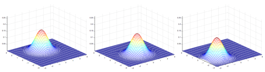
$$ Cov(X)=\Sigma $$The following examples are density plots of some Gaussian distributions, as shown in the figure below:
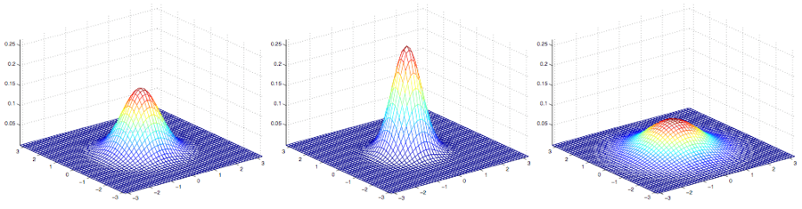
The leftmost plot shows a Gaussian distribution with mean $0$ (in fact a $2\times 1$ zero vector) and covariance matrix $\Sigma = I$ (a $2\times 2$ identity matrix). A Gaussian with mean $0$ and covariance equal to the identity matrix is also called the standard normal distribution. The middle plot shows the probability density of a Gaussian with mean $0$ and covariance $0.6I$; the rightmost plot shows the probability density of a Gaussian with covariance $\Sigma = 2I$. These figures show that as the covariance matrix $\Sigma$ grows, the Gaussian becomes more spread out, while if $\Sigma$ shrinks, the distribution becomes more compressed.
Here are some further examples:
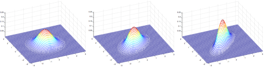
The plots above show Gaussian distributions with mean $0$ but with different covariance matrices, which are, in order:
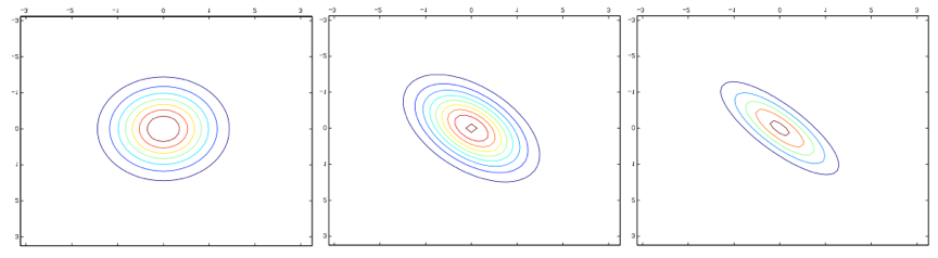
$$ \Sigma =\begin{bmatrix} 1 & 0 \\ 0 & 1 \\ \end{bmatrix}; \Sigma =\begin{bmatrix} 1 & 0.5 \\ 0.5 & 1 \\ \end{bmatrix}; \Sigma =\begin{bmatrix} 1 & 0.8 \\ 0.8 & 1 \\ \end{bmatrix} $$The first figure still looks much like the standard normal we saw earlier. We then find that, as the off-diagonal entries of the covariance matrix $\Sigma$ are increased, the density plot is gradually compressed toward the $45^\circ$ direction (that is, the direction in which $x_1 = x_2$). This is even clearer if we look at the contour plots of the same three densities:
The following is another set of examples, in which the covariance matrix $\Sigma$ has been adjusted:
$$ \Sigma =\begin{bmatrix} 1 & 0.5 \\ 0.5 & 1 \\ \end{bmatrix}; \Sigma =\begin{bmatrix} 1 & 0.8 \\ 0.8 & 1 \\ \end{bmatrix} \Sigma =\begin{bmatrix} 3 & 0.8 \\ 0.8 & 1 \\ \end{bmatrix}; $$The covariance matrices corresponding to the three figures above are as follows:
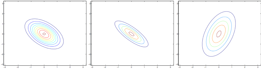
From the leftmost figure to the middle one (Translator’s note: note that in both the left and the middle of these covariance matrices, the upper-right and lower-left entries are negative!), it is clear that as the entries along the upper-right to lower-left diagonal of the covariance matrix decrease, the figure is compressed again, only in the opposite direction. Finally, as we change the parameters, the contours that are produced are usually ellipses (the rightmost figure is an example).
As a further set of examples, fix the covariance matrix to be the identity, that is, $\Sigma = I$, and then adjust the mean $\mu$. We can then shift the density plot along with the mean:
In every figure above the covariance matrix is the identity, that is, $\Sigma = I$, and the corresponding means $\mu$ are as follows:
$$ \mu =\begin{bmatrix} 1 \\ 0 \\ \end{bmatrix}; \mu =\begin{bmatrix} -0.5 \\ 0 \\ \end{bmatrix}; \mu =\begin{bmatrix} -1 \\ -1.5 \\ \end{bmatrix}; $$1.2 The Gaussian Discriminant Analysis Model
Suppose we have a classification problem in which the input features $x$ are continuous-valued random variables. We can then use the Gaussian discriminant analysis model (GDA), in which $p(x|y)$ is modeled by a multivariate normal distribution. The model is:
$$ \begin{aligned} y & \sim Bernoulli(\phi)\\ x|y = 0 & \sim N(\mu_o,\Sigma)\\ x|y = 1 & \sim N(\mu_1,\Sigma)\\ \end{aligned} $$Written out, the distributions are:
$$ \begin{aligned} p(y) & =\phi^y (1-\phi)^{1-y}\\ p(x|y=0) & = \frac{1}{(2\pi)^{n/2}|\Sigma|^{1/2}} exp ( - \frac{1}{2}(x-\mu_0)^T\Sigma^{-1}(x-\mu_0) )\\ p(x|y=1) & = \frac{1}{(2\pi)^{n/2}|\Sigma|^{1/2}} exp ( - \frac{1}{2}(x-\mu_1)^T\Sigma^{-1}(x-\mu_1) )\\ \end{aligned} $$In the equations above, the parameters of the model are $\phi, \Sigma, \mu_0$ and $\mu_1$. (Note that, although there are two distinct mean vectors $\mu_0$ and $\mu_1$, the model still generally uses only a single covariance matrix $\Sigma$.) The log-likelihood is as follows:
$$ \begin{aligned} l(\phi,\mu_0,\mu_1,\Sigma) &= \log \prod^m_{i=1}p(x^{(i)},y^{(i)};\phi,\mu_0,\mu_1,\Sigma)\\ &= \log \prod^m_{i=1}p(x^{(i)}|y^{(i)};\mu_0,\mu_1,\Sigma)p(y^{(i)};\phi)\\ \end{aligned} $$Maximizing $l$ gives the corresponding parameters, and those parameters are the maximum likelihood estimates, as follows (see Problem Set 1):
$$ \begin{aligned} \phi & = \frac {1}{m} \sum^m_{i=1}1\{y^{(i)}=1\}\\ \mu_0 & = \frac{\sum^m_{i=1}1\{y^{(i)}=0\}x^{(i)}}{\sum^m_{i=1}1\{y^{(i)}=0\}}\\ \mu_1 & = \frac{\sum^m_{i=1}1\{y^{(i)}=1\}x^{(i)}}{\sum^m_{i=1}1\{y^{(i)}=1\}}\\ \Sigma & = \frac{1}{m}\sum^m_{i=1}(x^{(i)}-\mu_{y^{(i)}})(x^{(i)}-\mu_{y^{(i)}})^T\\ \end{aligned} $$Pictorially, the algorithm can be represented as in the figure below:
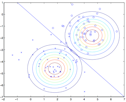
The points in the figure are the training set, and the two Gaussians are the separate fits to the two classes. Note that the contours of the two Gaussians have the same shape and the same direction of stretch, because they share the same covariance matrix $\Sigma$, but they have different means $\mu_0$ and $\mu_1$. In addition, the straight line in the figure is the decision boundary $p (y = 1|x) = 0.5$. On one side of this boundary we predict that $y = 1$ is the most likely outcome, and on the other side we predict that $y = 0$ is the most likely outcome.
1.3 Discussion: Gaussian Discriminant Analysis (GDA) and Logistic Regression
The Gaussian discriminant analysis model is interestingly related to logistic regression. If we view the quantity $p (y = 1|x; \phi, \mu_0, \mu_1, \Sigma)$ as a function of $x$, we find that it can be expressed in the following form:
$$ p(y=1|x;\phi,\Sigma,\mu_0,\mu_1)=\frac 1 {1+exp(-\theta^Tx)} $$where $\theta$ is some function of $\phi$, $\Sigma$, $\mu_0$, and $\mu_1$. This is the form that logistic regression (also a discriminative learning algorithm) uses to model $p (y = 1|x)$.
Note: The step above uses a transformation that redefines the vector $x^{(i)}$ by adding an extra coordinate $x_0^{(i)} = 1$ on the right-hand side, making it an $(n+1)$-dimensional vector. See Problem Set 1 for the details.
Which of these two models should we choose, and when? In general, Gaussian discriminant analysis (GDA) and logistic regression may give different decision boundaries on the same training set. Which one is better?
We have just shown that if $p(x|y)$ is a multivariate Gaussian distribution (with a shared covariance matrix $\Sigma$), then $p(y|x)$ must follow a logistic function. The converse, however, does not hold. For example, if $p(y|x)$ is a logistic function, that does not guarantee that $p(x|y)$ is a multivariate Gaussian. This shows that the Gaussian discriminant model makes stronger modeling assumptions about the data than logistic regression does. It also means that when the assumptions of both models are available, Gaussian discriminant analysis is better at fitting the data; it is the better model. In particular, when $p(x|y)$ is known to be Gaussian (with a shared covariance matrix $\Sigma$), Gaussian discriminant analysis is asymptotically efficient. In practice this also means that, faced with a very large training set (when the sample size $m$ is especially large), strictly speaking no other algorithm is likely to do better than Gaussian discriminant analysis (for example, in the accuracy of the estimate of $p(y|x)$). In that situation, then, Gaussian discriminant analysis (GDA) is a better algorithm than logistic regression. Extending the point a little further, even for small training sets we ultimately find that GDA is better.
There is, however, another side to the story. Because the assumptions made by logistic regression are significantly weaker, the decisions it gives are also more robust, and it is less sensitive to incorrect modeling assumptions. Many different sets of assumptions can lead $p(y|x)$ to a logistic function. For example, if $x|y = 0\sim Poisson(\lambda_0)$ is a Poisson distribution and $x|y = 1\sim Poisson(\lambda_1)$ is also a Poisson distribution, then $p(y|x)$ will be logistic as well. Logistic regression also applies to Poisson data of this kind. If, on such data, we insist on using Gaussian discriminant analysis (GDA) and fit a Gaussian to this non-Gaussian data, the predictability of the result falls, and GDA may work or it may not.
To sum up: Gaussian discriminant analysis (GDA) makes stronger modeling assumptions and uses data more efficiently (for example, it needs a smaller training set to achieve a “reasonably good” result), provided the modeling assumptions are correct or at least close to correct. Logistic regression makes weaker assumptions and is therefore more robust to departures from the modeling assumptions. If, however, the training data really are non-Gaussian, then in the limit of large data sets logistic regression is almost always better than GDA. In practice, therefore, logistic regression is used much more often than GDA. (The discussion comparing discriminative and generative models also applies to the naive Bayes algorithm that we turn to next, but naive Bayes is still regarded as an excellent and very popular classification algorithm.)
2 Naive Bayes
In Gaussian discriminant analysis (GDA), the feature vector $x$ is a continuous, real-valued vector. We now discuss another learning algorithm, for use when the $x_i$ are discrete.
Let us return to an example we have seen before, and try to build an email filter using machine learning. This time we classify email messages as commercial advertisements (that is, spam) or non-spam. Once we have learned how to implement this, we can have a mail reader automatically filter junk messages, or place that junk in a folder of its own. Classifying email is one case of the broader family of text-classification problems.
Suppose we have a training set (a pile of emails already labeled as spam or not). To build a spam filter, we begin by deciding which features $x_i$ will describe an email.
We represent an email by a feature vector whose length equals the number of words in the dictionary. If the email contains the $i$-th word in the dictionary, we set $x_i = 1$; otherwise $x_i = 0$. For example, the vector
$$ x=\begin{bmatrix}1\\0\\0\\\vdots \\1\\ \vdots \\0\end{bmatrix} \begin{matrix}\text{a}\\ \text{aardvark}\\ \text{aardwolf}\\ \vdots\\ \text{buy}\\ \vdots\\ \text{zygmurgy}\\ \end{matrix} $$represents an email that contains the two words “a” and “buy”, but not the words “aardvark”, “aardwolf”, or “zymurgy”. The set of words encoded into this feature vector is called the vocabulary, so the dimension of the feature vector $x$ equals the length of the vocabulary.
Note: In practice there is no need to walk through an entire English dictionary in order to build a list of every English word. The more common approach is to pass through the training set and encode into the feature vector only those words that appear more than once. Besides shortening the vocabulary in the model, this reduces the amount of computation and the space used. A further benefit is that the vocabulary can include words that appear in your email but not in a dictionary, such as the course abbreviation CS229. Sometimes (for example, in the homework) one also excludes especially high-frequency words, such as the article “the” and words like “of” and “and”. These high-frequency function words, which carry no specific meaning, are called stop words: they occur in a great many documents, and they are essentially useless for deciding whether an email is spam.
Once the feature vector has been chosen, the next step is to build a generative model. We must therefore model $p(x|y)$. But if we have fifty thousand words, then $x \in \{0, 1\}^{50000}$ (that is, $x$ is a $50000$-dimensional vector whose entries are $0$ or $1$). If we were to model such an $x$ with a multinomial distribution, there would be $2^{50000}$ possible outcomes, and we would need a parameter vector of dimension $(2^{50000}-1)$. That is clearly far too many parameters.
To model $p(x|y)$, we begin by making a very strong assumption. We assume that the features $x_i$ are independent given $y$. This assumption is called the naive Bayes assumption (the NB assumption), and the algorithm derived from it is called the naive Bayes classifier. For example, if $y = 1$ means that an email is spam, “buy” is word number $2087$, and “price” is word number $39831$, then we assume the following: if I tell you that $y = 1$, that is, that one particular email is spam, then knowing $x_{2087}$ (whether the word “buy” appears in the email) does not affect the credence you assign to $x_{39831}$ (whether the word “price” appears). More formally, this can be written $p(x_{2087}|y) = p(x_{2087}|y, x_{39831})$. (Note that this does not say that the two features $x_{2087}$ and $x_{39831}$ are independent, which would instead be $p(x_{2087}) = p(x_{2087}|x_{39831})$. What we are saying is that the two are conditionally independent given $y$.)
We then obtain the equation
$$ \begin{aligned} p(x_1, ..., x_{50000}|y) & = p(x_1|y)p(x_2|y,x_1)p(x_3|y,x_1,x_2) ... p(x_{50000}|y,x_1,x_2,...,x_{49999})\\ & = p(x_1|y)p(x_2|y)p(x_3|y) ... p(x_{50000}|y)\\ & = \prod^n_{i=1}p(x_i|y)\\ \end{aligned} $$The equality in the first line comes simply from the basic properties of probability, and the second equality uses the naive Bayes assumption. Note that the naive Bayes assumption is a strong one, yet the algorithm it produces applies to many kinds of problems.
The parameters of this model are $\phi_{i|y=1} = p (x_i = 1|y = 1)$, $\phi_{i|y=0} = p (x_i = 1|y = 0)$, and $\phi_y = p (y = 1)$. As before, given a training set $\{(x^{(i)},y^{(i)}); i = 1, ..., m\}$, we can write the joint likelihood as follows:
$$ \mathcal{L}(\phi_y,\phi_{j|y=0},\phi_{j|y=1})=\prod^m_{i=1}p(x^{(i)},y^{(i)}) $$The parameter values $\phi_y$, $\phi_{i|y=0}$, and $\phi_{i|y=1}$ that maximize the joint likelihood give the maximum likelihood estimates:
$$ \begin{aligned} \phi_{j|y=1} &=\frac{\sum^m_{i=1}1\{x_j^{(i)} =1 \wedge y^{(i)} =1\} }{\sum^m_{i=1}1\{y^{(i)} =1\}} \\ \phi_{j|y=0} &= \frac{\sum^m_{i=1}1\{x_j^{(i)} =1 \wedge y^{(i)} =0\} }{\sum^m_{i=1}1\{y^{(i)} =0\}} \\ \phi_{y} &= \frac{\sum^m_{i=1}1\{y^{(i)} =1\}}{m}\\ \end{aligned} $$In the equations above, the symbol “$\wedge$” (and) means logical “and”. These parameters have a very natural interpretation. For example, $\phi_{j|y=1}$ is exactly the fraction, among spam emails $(y = 1)$, of those emails in which word $j$ appears.
After all of these parameters have been fit, predicting for the feature vector $x$ of a new example requires only the following simple calculation:
$$ \begin{aligned} p(y=1|x)&= \frac{p(x|y=1)p(y=1)}{p(x)}\\ &= \frac{(\prod^n_{i=1}p(x_i|y=1))p(y=1)}{(\prod^n_{i=1}p(x_i|y=1))p(y=1)+ (\prod^n_{i=1}p(x_i|y=0))p(y=0)} \\ \end{aligned} $$and then choosing the class with the highest posterior probability.
Finally, note that in the use of naive Bayes just described, the features $x_i$ were all binary. Features may in fact take several discrete values, for example $\{1, 2, ..., k_i\}$. In that case we only need to change the model of $p(x_i|y)$ from a Bernoulli distribution to a multinomial distribution. Indeed, even if some of the original inputs are continuous (for example, living area in our first example), they can be converted into a small set of discrete values and then used with naive Bayes. For example, if we use a feature $x_i$ to represent living area, we can discretize that variable as follows:
| Living area | $<400$ | $400-800$ | $800-1200$ | $1200-1600$ | $>1600$ |
|---|---|---|---|---|---|
| Discrete value $x_i$ | $1$ | $2$ | $3$ | $4$ | $5$ |
Thus, for a house of area $890$ square feet, we set this component $x_i$ of the feature vector to $3$, according to the corresponding value in the set above. We can then apply the naive Bayes algorithm and model $p(x_i|y)$ as a multinomial distribution, just as in the discussion above. When an originally continuous attribute is not easy to model with a multivariate normal distribution, discretizing its feature and using naive Bayes (NB) in place of Gaussian discriminant analysis (GDA) usually produces a better classifier.
2.1 Laplace Smoothing
The naive Bayes algorithm just described can already solve many problems, but a small adjustment can improve it further, especially for text classification. Let us briefly discuss a problem with the algorithm in its present form, and then how to fix that problem.
Consider again the process of classifying spam. Suppose you have finished CS229, carried out an excellent research project, and then decide, in June $2003$ (Translator’s note: the author must have written these notes quite early), to submit your work to the NIPS conference. NIPS is a top conference in machine learning, and the paper deadline is usually from the end of June to the beginning of July. You discuss the conference by email, and you also begin to receive messages containing the four letters nips. But this is your first NIPS paper, and before this you had never received any email containing the word nips. What matters especially is that the word nips has never appeared in your spam/non-spam training set. Suppose nips is the $35000$-th word in your dictionary. Your naive Bayes spam filter then forms the maximum likelihood estimate of the parameter $\phi_{35000|y}$ as follows:
$$ \begin{aligned} \phi_{35000|y=1} &= \frac{\sum^m_{i=1}1\{x^{(i)}_{35000}=1 \wedge y^{(i)}=1 \}}{\sum^m_{i=1}1\{y^{(i)}=0\}} &=0 \\ \phi_{35000|y=0} &= \frac{\sum^m_{i=1}1\{x^{(i)}_{35000}=1 \wedge y^{(i)}=0 \}}{\sum^m_{i=1}1\{y^{(i)}=0\}} &=0 \\ \end{aligned} $$That is, because the program has never seen the word nips in any other spam or non-spam training example, it takes the probability of seeing this word in either kind of email to be $0$. So when it must decide whether an email containing the word nips is spam, it checks the posterior probability of the class and obtains
$$ \begin{aligned} p(y=1|x) &= \frac{ \prod^n_{i=1} p(x_i|y=1)p(y=1) } {\prod^n_{i=1} p(x_i|y=1)p(y=1) +\prod^n_{i=1} p(x_i|y=0)p(y=0) }\\ &= \frac00\\ \end{aligned} $$This is because every product “$\prod^n_{i=1} p(x_i|y)$” that includes $p(x_{35000}|y) = 0$ collapses to $0$ as well. Our algorithm therefore obtains $\frac00$, which means it does not know what prediction to make.
Pushing the problem one step further: statistically, it is clearly not a good idea to estimate the probability of an event as zero merely because you have never seen it in your own previous, finite training set. Suppose the problem is to estimate a multinomial random variable $z$ taking values in $\{1,..., k\}$. We can then take $\phi_i = p (z = i)$ as the multinomial parameters. Given a set of $m$ independent observations $\{z^{(1)}, ..., z^{(m)}\}$, the maximum likelihood estimate has the following form:
$$ \phi_j=\frac{\sum^m_{i=1}1\{z^{(i)}=j\}}m $$As we saw earlier, if we use these maximum likelihood estimates, some $\phi_j$ may end up equal to zero, and that is a problem. To avoid this situation, we introduce Laplace smoothing, which replaces the estimate above by
$$ \phi_j=\frac{\sum^m_{i=1}1\{z^{(i)}=j\}+1}{m+k} $$Here we first add $1$ to the numerator and then add $k$ to the denominator. Note that $\sum^k_{j=1} \phi_j = 1$ still holds (check this yourself). That is a property we must have, because the $\phi_j$ are estimates of probabilities, and all the probabilities added together must equal $1$. In addition, $\phi_j \neq 0$ for every value of $j$, which solves the problem of a probability estimate being zero. Under certain conditions (arguably quite strong assumptions), Laplace smoothing can in fact be shown to give the optimal estimator of the parameters $\phi_j$.
Returning to our naive Bayes filter, once Laplace smoothing is used the estimates of the parameters are written as follows:
$$ \begin{gathered} \phi_{j|y=1} =\frac{\sum_{i=1}^m1\{x_j^{(i)}=1\wedge y^{(i)}=1\}+1}{\sum_{i=1}^m1\{y^{(i)}=1\}+2} \\ \phi_{j|y=0} =\frac{\sum_{i=1}^m1\{x_j^{(i)}=1\wedge y^{(i)}=10\}+1}{\sum_{i=1}^m1\{y^{(i)}=0\}+2} \end{gathered} $$(In practice, whether or not Laplace smoothing is applied to $\phi_y$ usually does not matter much, because we typically have a suitable proportion of both spam and non-spam emails, so $\phi_y$ is a reasonable estimate of $p(y = 1)$ and, either way, stays some distance away from zero.)
2.2 Event Models for Text Classification
This is a good place to bring our discussion of generative learning algorithms to a close, so we continue with another model for text classification. The naive Bayes method we have just demonstrated can already solve many classification problems, but there is another related algorithm that does still better at classifying text.
In the particular setting of text classification, the naive Bayes method above uses what is called the multivariate Bernoulli event model. In this model we assume that the way an email is sent is determined at random (according to the class prior $p(y)$): whether or not the sender is a spammer, whether that sender sends you the next email is decided at random. The sender then walks through the dictionary and decides whether to include each word $i$ in the email. The words are independent of one another and follow the distribution $p(x_i=1|y)=\phi_{i|y}$. The probability of a message is therefore $p(y)\prod^n_{i-1}p(x_i|y)$.
There is another model, called the multinomial event model. To describe it, we need a different notation and a different set of features for representing emails. Let $x_i$ denote the $i$-th word in the message. Thus $x_i$ is now an integer taking values in $\{1,...,|V|\}$, where $|V|$ is the length of the vocabulary (that is, the dictionary). An email of $n$ words can then be represented as a vector $(x_1,x_2,...,x_n)$ of length $n$; note that $n$ can take different values for different emails. For example, if an email begins “A NIPS . . .”, then $x_1 = 1$ (“a” is the first word in the dictionary) and $x_2 = 35000$ (assuming that “nips” is the 35000th word in the dictionary).
In the multinomial event model we assume that an email is generated by a random process, and that whether it is spam is decided first (according to $p(y)$), just as in the assumptions of the previous model. The sender then writes the email by first generating $x_1$ from some multinomial distribution over words, $(p(x_1|y))$. The second step generates $x_2$ independently of $x_1$, but drawn from the same multinomial distribution, and likewise $x_3$, $x_4$, and so on, until every word in the email has been generated. The overall probability of an email is therefore $p(y)\prod^n_{i=1}p(x_i|y)$. Note that this equation looks very similar to the message probability in the multivariate Bernoulli event model above, but the meaning is entirely different. In particular, $x_i|y$ is now a multinomial distribution rather than a Bernoulli distribution.
The parameters of our new model are still $\phi_y = p(y)$, as before, together with $\phi_{k|y=1} = p(x_j =k|y=1)$ (for any $j$) and $\phi_{i|y=0} =p(x_j =k|y=0)$. Note that we have assumed that the probability $p(x_j|y)$ is the same for every value of $j$, which means that the distribution generating the words does not depend on the position $j$ of the word in the email.
Given a training set $\{(x^{(i)},y^{(i)}); i = 1, ..., m\}$, where $x^{(i)} = ( x^{(i)}_{1} , x^{(i)}_{2} ,..., x^{(i)}_{n_i})$ (here $n_i$ is the number of words in the $i$-th training example), the likelihood of the data is as follows:
$$ \begin{aligned} \mathcal{L}(\phi,\phi_{k|y=0},\phi_{k|y=1})& = \prod^m_{i=1}p( x^{(i)},y^{(i)})\\ & = \prod^m_{i=1}(\prod^{n_i}_{j=1}p(x_j^{(i)}|y;\phi_{k|y=0},\phi_{k|y=1}))p( y^{(i)};\phi_y)\\ \end{aligned} $$Maximizing the function above yields the maximum likelihood estimates of the parameters:
$$ \begin{aligned} \phi_{k|y=1}&= \frac{\sum^m_{i=1}\sum^{n_i}_{j=1}1\{x_j^{(i)}=k\wedge y^{(i)}=1\}}{\sum^m_{i=1}1\{y^{(i)}=1\}n_i} \\ \phi_{k|y=0}&= \frac{\sum^m_{i=1}\sum^{n_i}_{j=1}1\{x_j^{(i)}=k\wedge y^{(i)}=0\}}{\sum^m_{i=1}1\{y^{(i)}=0\}n_i} \\ \phi_y&= \frac{\sum^m_{i=1}1\{y^{(i)}=1\}}{m}\\ \end{aligned} $$If Laplace smoothing is used (as it is in practice, to improve performance) to estimate $\phi_{k|y=0}$ and $\phi_{k|y=1}$, we add $1$ to the numerator and $|V|$ to the denominator, and obtain the following equations:
$$ \begin{aligned} \phi_{k|y=1}&= \frac{\sum^m_{i=1}\sum^{n_i}_{j=1}1\{x_j^{(i)}=k\wedge y^{(i)}=1\}+1}{\sum^m_{i=1}1\{y^{(i)}=1\}n_i+|V|} \\ \phi_{k|y=0}&= \frac{\sum^m_{i=1}\sum^{n_i}_{j=1}1\{x_j^{(i)}=k\wedge y^{(i)}=0\}+1}{\sum^m_{i=1}1\{y^{(i)}=0\}n_i+|V|} \\ \end{aligned} $$This is not necessarily the best classification algorithm, of course, but naive Bayes classifiers usually work surprisingly well. The method is therefore a very good “first choice”, because it is simple and easy to implement.