
Chapter 4
Part 6: Learning Theory
1 The bias/variance tradeoff
When we discussed linear regression, we considered the following question: when fitting the data, should we choose a “simple” model such as the linear model “$y = \theta_0 +\theta_1x$”, or a “complex” model such as the polynomial “$y= \theta_0 + \theta_1x+ ...+\theta_5x^5$”? This is illustrated below:
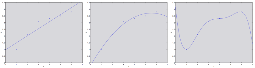
As the rightmost plot shows, fitting with a fifth-degree polynomial does not yield a good model. Moreover, although this fifth-degree polynomial gives a very good predicted value of $y$ (the corresponding housing price) for every $x$ in the training set (for example, the living area mentioned earlier in the notes), we still cannot expect this model to give reliable predictions for points outside the training set. In other words, a model obtained by learning from the training set with a high-degree polynomial of this kind simply does not carry over to other houses. The generalization error of a hypothesis (a formal definition will be given shortly) is precisely the expected error on examples that are not necessarily in the training set.
In the figure above, both the linear fit on the far left and the high-degree polynomial fit on the far right have very large generalization error. The problems with these two models, however, are quite different. If the relationship between $y$ and $x$ is not linear, then even if we have a very large training set and use it to fit a line, the resulting linear model still cannot accurately capture the structure of the data. We informally define the bias of a model to be its expected generalization error, even when what we are fitting is a very large, or even infinite, training set. In that sense, for the situation shown in the three plots above, the linear model on the far left has especially large bias, and may be underfitting the data (that is, failing to capture the structural features present in the data).
Besides this bias, there is another ingredient of the generalization error: the variance of the fitting process. In the rightmost plot, for example, a fifth-degree polynomial is used. This carries a large risk. The model we fit from the data may happen to suit only the small, finite training set at hand, and may not reflect the broader relationship between $x$ and $y$. In practice, the houses in the training set we happened to choose might be somewhat more expensive than average, or some of them might be a bit cheaper than average, and so on. By fitting such a “spurious” pattern in the training set, we may obtain a model with large generalization error. In that case, we say that the model has large variance.$^1$
1 In these notes we do not intend to give formal definitions of bias and variance; the discussion above is as far as we will go. Of course, both notions do have strict formal definitions. In linear regression, for example, there are several different views of how the two should be defined, and which of them is the most authoritative and the most correct is still debated.
In general, we have to compromise between bias and variance. If our model is too “simple” and has very few parameters, it may have large bias while the variance is small. If our model is too “complex” and has a great many parameters, the situation may be reversed: the variance may be especially large, while the bias is smaller. Among the three fits in the example above, the quadratic fit is clearly better than the straight-line fit, and also better than the fifth-degree polynomial fit.
2 Preliminaries
In this part of the notes, we begin learning theory. The material in this chapter is very interesting and suggestive, and it helps us build intuition and rules of thumb for how best to apply learning algorithms in different settings. We will also look into several questions. First, can the bias/variance tradeoff we have just discussed be summarized more formally? This question also leads to methods for model selection, which can help determine, while fitting a training set, what degree the polynomial should have. Second, what we truly care about in machine learning is the generalization error, yet most learning algorithms work by fitting a model to a training set. Why, then, should performance on the training set tell us anything about the generalization error? For example, can we relate the error on the training set to the generalization error? Third, and finally, are there conditions under which we can prove that certain learning algorithms work well?
We begin with two very simple and very useful lemmas.
Lemma 1 (The union bound). Let $A_1, A_2, ..., A_k$ be $k$ events (not necessarily mutually independent). Then:
$$ P(A_1\cup...\cup A_k)\leq P(A_1)+...+P(A_k) $$In probability, the union bound is usually taken as an axiom (so we will not try to prove it). It is also quite intuitive: the probability that at least one of $k$ events occurs is at most the sum of the probabilities that the $k$ events occur individually.
Lemma 2 (Hoeffding’s inequality). Let $Z_1,...,Z_m$ be $m$ independent and identically distributed (iid) random variables, all following a Bernoulli($\phi$) distribution. For example, $P(Z_i =1)=\phi$ and $P(Z_i =0)= 1 - \phi$. Let $\hat\phi=(\frac1m)\sum^m_{i=1}Z_i$ be the mean of these random variables, and let $\gamma \geq 0$ be an arbitrary fixed value. Then:
$$ P(|\phi-\hat\phi|>\gamma)\leq 2\exp (-2\gamma^2m) $$This lemma (also called the Chernoff bound in learning theory) says that if we take the mean $\hat\phi$ of random variables drawn from a Bernoulli distribution as an estimate of $\phi$, then as long as $m$ is large enough, the probability of deviating far from the true value is small. Another way to put it: if you have a biased coin whose probability of landing heads is $\phi$, and you toss it $m$ times and compute the fraction of heads, then when $m$ is very large that fraction is, with high probability, a good estimate of $\phi$.
Using these two lemmas, we can prove some deep and important results in learning theory.
To simplify the presentation, we first focus on binary classification, in which the labels are simply $y \in \{0, 1\}$. Everything we are about to discuss also extends to other problems, such as regression and multiclass classification.
Suppose we are given a training set $S = \{(x^{(i)},y^{(i)});i = 1,...,m\}$ of sample size $m$, in which the training examples $(x^{(i)},y^{(i)})$ are iid random variables drawn from some probability distribution $D$. Let $h$ be a hypothesis. We define the training error (also called the empirical risk or the empirical error in learning theory) as follows:
$$ \hat\epsilon(h) =\frac1m\sum^m_{i=1}1\{h(x^{(i)})\neq y^{(i)}\} $$This value is simply the fraction of the training examples that the hypothesis $h$ misclassifies. When we want to make explicit the empirical error $\hat\epsilon(h)$ on a particular training set $S$, we may write $\hat\epsilon_S(h)$. We then define the generalization error as:
$$ \epsilon(h) =P_{(x,y)\sim D}(h(x)\neq y) $$Under this definition, the generalization error $\epsilon(h)$ is exactly the probability that the hypothesis $h$ misclassifies a new example $(x, y)$ drawn from the distribution $D$.
Note that we are assuming in advance that the training data and the data used to test the hypothesis are drawn from the same distribution $D$ (this assumption is present in the definition of the generalization error). This assumption is usually regarded as one of the PAC assumptions.$^2$
2 PAC is an abbreviation of “probably approximately correct.” It is a framework, together with a collection of assumptions, and many results in learning theory are proved from these assumptions. The two most important assumptions in the collection are that the training set and the test set follow the same distribution, and that the training examples are independent.
Consider linear classification, and suppose $h_\theta (x) = 1\{\theta^T x \geq 0\}$. What is a reasonable way to fit the parameter $\theta$? One approach is to minimize the training error, and to take the $\theta$ at which the minimum is attained:
$$ \hat\theta=arg\min_\theta\hat\epsilon(h_\theta) $$We call this procedure empirical risk minimization (ERM for short), and the hypothesis obtained by the learning algorithm in this case is $\hat h = h_{\hat\theta}$. We regard ERM as the most “basic” learning algorithm, and it is the algorithm we focus on throughout this set of notes. (Other algorithms, such as logistic regression, can also be viewed as approximations to ERM.)
In our study of learning theory, it is useful to abstract away the specific parameterization, and also to abstract away questions such as whether a linear classifier is being used. We define the hypothesis class $H$ used by the learning algorithm to be the set of all classifiers under consideration. For linear classification, $H = \{h_\theta : h_\theta(x) = 1\{\theta^T x \geq 0\}, \theta \in R^{n+1}\}$ is the set of all classifiers of the input features $X$ whose decision boundaries are linear. More broadly, if we are studying neural networks, we may let $H$ be the set of all classifiers representable by some neural-network architecture.
Empirical risk minimization (ERM) can now be viewed as minimization over the function class $H$, in which the learning algorithm chooses the hypothesis:
$$ \hat h=arg\\min_{h\in H}\hat\epsilon(h) $$3 The case of finitely many hypotheses (finite $H$)
We first consider learning when the hypothesis class is finite, where the hypothesis class $H = \{h_1, ..., h_k\}$ consists of $k$ distinct hypotheses. Thus $H$ is a set of $k$ functions mapping the input features $X$ to $\{0, 1\}$, and empirical risk minimization (ERM) selects as $\hat h$ the one among these $k$ functions with the smallest training error.
We would like to guarantee something about the generalization error of $\hat{h}$. This takes two steps. First, show that $\hat\epsilon(h)$ is a reliable estimate of $\epsilon(h)$ for every $h$. Second, show that this $\hat\epsilon(h)$ upper-bounds the generalization error of $\hat{h}$.
Fix an arbitrary $h_i \in H$. Suppose $Z$ is a Bernoulli random variable whose distribution is defined as follows. We draw $(x, y)$ from $D$ and set $Z=1\{h_i(x)\neq y\}$. That is, we pick an example and let $Z$ indicate whether $h_i$ misclassifies that example. Similarly, we define $Z_j=1\{h_i(x^{(j)})\neq y^{(j)}\}$. Because our training examples are iid random variables drawn from $D$, the $Z$ and $Z_j$ constructed from them follow the same distribution.
We then find that the probability of misclassifying a randomly drawn training example — that is, $\epsilon(h)$ — is exactly the expected value of $Z$ (and of $Z_j$). The training error can therefore be written as:
$$ \hat\epsilon(h_i)=\frac 1m\sum_{j=1}^mZ_j $$Thus $\hat\epsilon(h_i)$ is exactly the average of the $m$ random variables $Z_j$, and these $Z_j$ are iid Bernoulli random variables whose mean is $\epsilon(h_i)$. Applying Hoeffding’s inequality, we obtain:
$$ P(|\epsilon(h_i)-\hat\epsilon(h_i)|>\gamma)\leq 2\exp (-2\gamma^2m) $$This shows that, for a given fixed $h_i$, when the training-set size $m$ is large, the training error is close to the generalization error with high probability. We are not content, however, with a high-probability guarantee that $\epsilon(h_i)$ is close to $\hat\epsilon(h_i)$ only for one particular $h_i$. We also want to prove that the conclusion holds simultaneously for every $h \in H$. To prove this, let $A_i$ denote the event $|\epsilon(h_i) - \hat\epsilon(h_i)| > \gamma$. We have already shown that $P(A_i) \le 2\exp (-2\gamma^2m)$ for any given $A_i$. Using the union bound, we then obtain:
$$ \begin{aligned} P(\exists h\in H.|\epsilon(h_i)-\hat\epsilon(h_i)|>\gamma)& = P(A_1\cup...\cup A_k) \\ & \le \sum_{i=1}^k P(A_i) \\ & \le \sum_{i=1}^k 2\exp (-2\gamma^2m) \\ & = 2k\exp (-2\gamma^2m) \end{aligned} $$If we subtract both sides from 1, the inequality reverses and becomes:
$$ \begin{aligned} P(\neg\exists h\in H.|\epsilon(h_i)-\hat\epsilon(h_i)|>\gamma)& = P(\forall h\in H.|\epsilon(h_i)-\hat\epsilon(h_i)|\le\gamma) \\ & \ge 1-2k\exp (-2\gamma^2m) \end{aligned} $$(The symbol “$\neg$” means “not.”) As shown above, with probability at least $1-2k\exp(-2\gamma^2 m)$, we can ensure that for every $h \in H$, $\epsilon(h)$ lies within $\gamma$ of $\hat\epsilon(h)$. A result of this kind is called a uniform convergence result, because it is a bound that holds for all $h \in H$ at once (as opposed to a bound that holds only for a single $h$).
In the discussion above, for certain particular values of $m$ and $\gamma$, we gave a probabilistic bound: for some $h \in H$, $|\epsilon(h) - \hat\epsilon(h)| \geq \gamma$. There are three quantities of interest here: $m$, $\gamma$, and the probability of error. We can bound any one of them in terms of the other two.
For example, we may ask the following question. Given $\gamma$ and some $\delta \geq 0$, how large must $m$ be if we want the probability that the training error lies within $\gamma$ of the generalization error to be at least $1-\delta$? Set $\delta = 2k\exp(-2\gamma^2 m)$ and solve for $m$ (prove to yourself that this is correct!). We then find that if
$$ m\ge \frac{1}{2\gamma^2}log\frac{2k}{\delta} $$then with probability at least $1-\delta$ we are guaranteed that $|\epsilon(h) - \hat\epsilon(h)| \le \gamma$ for every $h \in H$. (Equivalently, the probability that $|\epsilon(h) - \hat\epsilon(h)| \geq \gamma$ for some $h \in H$ is at most $\delta$.) This union bound also tells us how many training examples are needed before the result can be guaranteed. The training-set size $m$ that a particular method or algorithm needs in order to achieve a certain level of performance is called the sample complexity of that algorithm.
The key property of the bound above is that the number of training examples needed to guarantee the result is only logarithmic in $k$, where $k$ is the number of hypotheses in the hypothesis class $H$. This property will matter later.
In the same way, we can hold $m$ and $\delta$ fixed and solve the equation above for $\gamma$. This shows that, with probability $1-\delta$, the following holds for every $h \in H$ (again, you should prove this yourself, though it is fine simply to trust that it is correct):
$$ |\hat\epsilon(h)-\epsilon(h)|\le \sqrt{\frac{1}{2m}log\frac{2k}{\delta}} $$Now suppose that uniform convergence holds, that is, $|\epsilon(h)-\hat\epsilon(h)| \le \gamma$ for every $h \in H$. Our learning algorithm selects $\hat{h} = arg\\min_{h\in H} \hat\epsilon(h)$. What can we prove about the generalization of an algorithm of this kind?
Define $h^* = arg \\min_{h\in H} \epsilon(h)$ to be the best possible hypothesis in $H$. Note that this $h^*$ is the best hypothesis we can find using the hypothesis class $H$, so it is natural to use $h^*$ as the benchmark for performance. We then have:
$$ \begin{aligned} \epsilon(\hat h) & \le \hat\epsilon(\hat h)+\gamma \\ & \le \hat\epsilon(h^*)+\gamma \\ & \le \epsilon(h^*)+2\gamma \end{aligned} $$The first line uses the fact that $| \epsilon(\hat h) - \hat\epsilon (\hat h) | \le \gamma$ (which follows from the uniform-convergence assumption above). The second line uses the fact that $\hat{h}$ was chosen to minimize $\hat\epsilon(h)$, and therefore $\hat\epsilon(\hat{h}) \leq \hat\epsilon(h)$ for every $h$, which in particular gives $\hat\epsilon(\hat{h}) \le \hat\epsilon(h^*)$. The third line uses the uniform-convergence assumption once more; that assumption implies $\hat\epsilon(h^*) \le \epsilon(h^*) + \gamma$. We therefore conclude that if uniform convergence holds, then the generalization error of $\hat h$ differs from that of the best possible hypothesis in $H$ by at most $2\gamma$.
Let us now collect all of the above into a theorem.
Theorem: Let $|H| = k$. Translator’s note: that is, the number of elements in the set $H$ is $k$. Let $m$ and $\delta$ be arbitrary fixed values. Then, with probability at least $1 - \delta$,
$$ \epsilon(\hat h)\le (\\min_{h\in H}\epsilon(h))+2\sqrt{\frac{1}{2m}log\frac{2k}{\delta}} $$The proof is obtained by setting $\gamma$ equal to the square-root expression $\sqrt{\cdot}$, using the fact established earlier that uniform convergence holds with probability at least $1-\delta$, and then using uniform convergence to show that $\epsilon(h)$ exceeds $\epsilon(h^*) = \\min_{h\in H} \epsilon(h)$ by at most $2\gamma$ (which we have already proved).
This also gives a quantitative form of the bias/variance tradeoff in model selection that was mentioned earlier. Suppose, for example, that we have some hypothesis class $H$, and that we consider switching to some larger hypothesis class $H' \supseteq H$. If we switch to $H'$, the first term, $\min_h \epsilon(h)$, can only decrease, because we are now taking the minimum over a larger set of functions. Thus, if we learn with a larger hypothesis class, the “bias” of our learning algorithm can only decrease. If $k$ increases, however, the second term — twice the square root, $2\sqrt{\cdot}$ — also increases. The growth of this term means that when we use a larger hypothesis class, the “variance” increases.
Holding $\gamma$ and $\delta$ fixed and solving for $m$ as above, we also obtain the following sample-complexity bound:
Corollary: Let $|H| = k$, and let $\delta$ and $\gamma$ be arbitrary fixed values. For $\epsilon(\hat{h}) \le \min_{h\in H} \epsilon(h) + 2\gamma$ to hold with probability at least $1 - \delta$, the following relation holds:
$$ \begin{aligned} m &\ge \frac{1}{2\gamma^2}log\frac{2k}{\delta} \\ & = O(\frac{1}{\gamma^2}log\frac{k}{\delta}) \end{aligned} $$4 The case of infinitely many hypotheses (infinite $H$)
We have proved some useful theorems for finite hypothesis classes. Many hypothesis classes, however, contain infinitely many functions, including classes parameterized by real numbers (linear classification, for example). Can we prove similar results when there are infinitely many hypotheses?
We begin with an argument that is not quite the “right” one. There are of course better and more general arguments, but starting from this less “correct” argument will help build our intuition in this area.
Suppose we have a hypothesis class $H$ parameterized by $d$ real numbers. Because we represent real numbers on a computer, and an IEEE double-precision floating-point number (the double type in C) uses 64 bits to represent one floating-point number, a learning algorithm that uses double-precision floating point is parameterized by $64d$ bits. Such a hypothesis class therefore contains at most $k = 2^{64d}$ distinct hypotheses. Combining this with the corollary at the end of the previous section, we find that to guarantee $\epsilon(\hat{h}) \leq \epsilon(h^*) + 2\gamma$, and to guarantee that the probability is at least $1 - \delta$, the training-set size $m$ must satisfy $m \ge O(\frac{1}{\gamma^2}log\frac{2^{64d}}{\delta})=O(\frac{d}{\gamma^2}log\frac{1}{\delta})=O_{\gamma,\delta}(d)$ (the subscripts $\gamma$ and $\delta$ on the last big-$O$ mean that the hidden constant may depend on $\gamma$ and $\delta$). Therefore, the number of training examples needed is at most linear in the parameters of the model.
The argument above assumes that the parameters are 64-bit floating-point numbers, whereas real-valued parameters need not actually be implemented that way. The fact that we relied on 64-bit floating point makes this argument not entirely satisfying, but the conclusion is nonetheless roughly correct: If what we’re going to do is try to minimize training error, then in order to learn “well” using a hypothesis class that has $d$ parameters, generally we’re going to need on the order of a linear number of training examples in $d$.
(Note here that the conclusions above have been shown to apply to learning algorithms that use empirical risk minimization (ERM). A linear dependence of the sample complexity on $d$ therefore usually applies to most discriminative learning algorithms, whereas minimizing the training error, or an approximation to the training error, does not necessarily apply to discriminative learning. Giving reliable theoretical arguments for many non-ERM learning algorithms remains a very active area of research.)
Another unsatisfactory part of the preceding argument is that it depends on a parameterization of $H$. Intuitively, the parameterization ought not to matter much. We have written a linear classifier as $h_\theta(x) = 1\{\theta_0 + \theta_1x_1 + \cdot\cdot\cdot\theta_n x_n \geq 0\}$, which has $n+1$ parameters $\theta_0,...,\theta_n$. It can also be written as $h_{u,v}(x) = 1\{(u^2_0 - v_0^2) + (u^2_1 - v_1^2)x1 + \cdot\cdot\cdot (u^2_n - v_n^2)x_n \geq 0\}$, which has $2n+2$ parameters $u_i, v_i$. Both forms, however, define the same $H$: the set of linear classifiers in $n$ dimensions.
To reach a more satisfactory argument, we need a few additional definitions.
Given a set of points $S = \{x^{(i)}, ..., x^{(d)}\}$ (unrelated to the training set) with $x(i) \in X$, we say that $H$ shatters $S$ if $H$ can realize any labeling on $S$. That is, for every set of labels $\{y^{(1)}, ..., y^{(d)}\}$, there is some $h\in H$ such that $h(x^{(i)}) = y^{(i)}$ for all $i = 1, ...d$. (Translator’s note: for the definition of a shattered set, see https://en.wikipedia.org/wiki/Shattered_set. For more on the VC dimension, see also https://www.zhihu.com/question/38607822.)
Given a hypothesis class $H$, we define its VC dimension (Vapnik-Chervonenkis dimension), written $VC(H)$, to be the size of the largest set that $H$ can shatter. (If $H$ can shatter arbitrarily large sets, then $VC(H) = \infty$.)
For example, take a set consisting of the three points shown below:
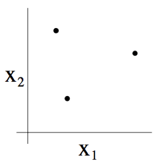
Can the class $H$ of two-dimensional linear classifiers $(h(x) = 1\{\theta_0 +\theta_1 x_1 + \theta_2 x_2 \geq 0\})$ shatter the set in the figure? Yes. Concretely, as the next figure shows, for any one of the eight labelings we can find a linear classifier that achieves zero training error:
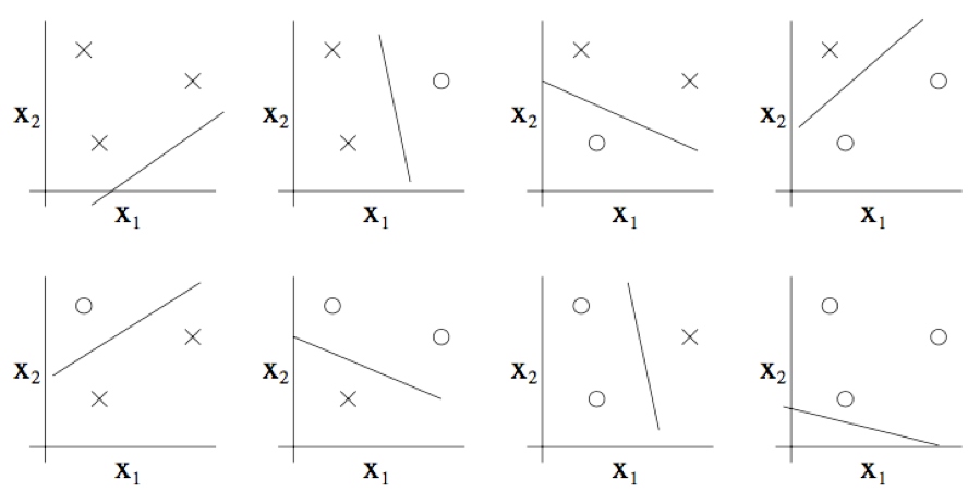
It can also be shown that this hypothesis class $H$ cannot shatter a set of 4 points. The largest set that $H$ can shatter therefore has size 3, that is, $VC(H) = 3$.
Note that the VC dimension of $H$ is 3 even though some sets of 3 points cannot be shattered by $H$. If, for example, the three points lie on a straight line (as in the left plot below), no linear classifier can separate all possible labelings of those three points (as suggested on the right).
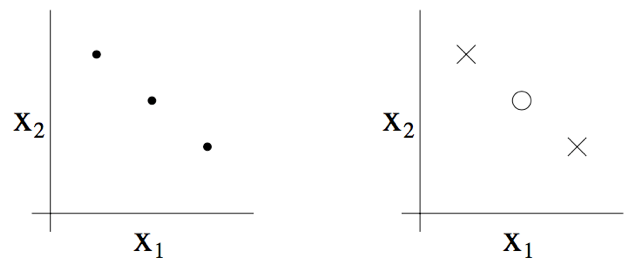
Put another way, under the definition of the VC dimension, to ensure that $VC(H)$ is at least $d$ it is enough to prove that at least one set of size $d$ can be shattered by $H$.
This brings us to the following theorem, due to Vapnik. (Many people regard it as the single most important theorem in all of learning theory.)
Theorem. Let $H$ be given, and let $d = VC(H)$. Then with probability at least $1-\delta$, we have that for all $h \in H$,
$$ |\epsilon(h)-\hat\epsilon(h)|\le O(\sqrt{\frac{d}{m}log\frac{d}{m}+\frac 1mlog\frac 1\delta}) $$Moreover, with probability at least $1-\delta$,
$$ \epsilon(\hat h)\le \epsilon(h^*)+O(\sqrt{\frac{d}{m}log\frac{d}{m}+\frac 1mlog\frac 1\delta}) $$In other words, if a hypothesis class has finite VC dimension, then as the training-set size $m$ grows we are guaranteed that uniform convergence occurs. As before, this lets us place a bound on $\epsilon(h^*)$ in terms of $\epsilon(h)$. There is also the following corollary:
Corollary. For $|\epsilon(h) - \hat\epsilon(h)| \le \gamma$ to hold for all $h \in H$ (and hence $\epsilon(\hat{h}) \le \epsilon(h^*) + 2\gamma$) with probability at least $1-\delta$, it suffices that $m = O_{\gamma,\delta}(d)$.
In other words, the number of training examples needed to learn “well” using H is linear in the VC dimension of H. It turns out that, for “most” hypothesis classes, the VC dimension (assuming a “reasonable” parameterization) is also roughly linear in the number of parameters. Putting these together, we conclude that (for an algorithm that tries to minimize training error) the number of training examples needed is usually roughly linear in the number of parameters of H.