
Chapter 1
Supervised Learning
Let us begin with a few examples of solving problems with supervised learning. Suppose we have a data set containing the living area and price of $47$ houses in Portland, Oregon:
| Living area (square feet) | Price (thousands of dollars) |
|---|---|
| $2104$ | $400$ |
| $1600$ | $330$ |
| $2400$ | $369$ |
| $1416$ | $232$ |
| $3000$ | $540$ |
| $\vdots$ | $\vdots$ |
Plot these data:
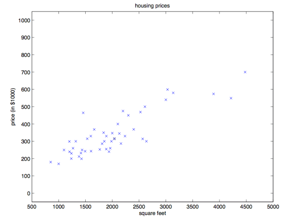
Given data like these, how can we learn to predict the prices of other houses in Portland, together with their living areas?
We first need to fix some notation that we will keep using. Let $x^{(i)}$ denote the “input” variables (living area in this example), also called the input features. Let $y^{(i)}$ denote the “output,” or the target variable, which in this example is the house price. A pair $(x^{(i)},y^{(i)})$ is called a training example, and the data set we use to let the machine learn — a list of $m$ training examples, $\{(x^{(i)},y^{(i)}); i = 1,\dots ,m\}$ — is called a training set. Note carefully that the superscript $(i)$ is only an index into the training set. It has nothing to do with exponentiation; do not misread it. We will also use an uppercase $X$ for the space of input values and an uppercase $Y$ for the space of output values. In the example of this section both spaces are the real numbers, so $X = Y = R$.
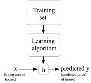
To state the supervised learning problem more formally: given a training set, our goal is to have the machine learn a function $h: X \to Y$ so that $h(x)$ is an estimate reasonably close to the corresponding true value of $y$. For historical reasons, this function $h$ is called a hypothesis. Pictorially, the process looks roughly like this:
When the target variable we want to predict is continuous, as in this house price–area example, the learning problem is called a regression problem. When $y$ can take only a small number of discrete values (for example, given the living area, we want to decide whether the house is a residence or an apartment), the problem is called a classification problem.
Part I: Linear Regression
To make the housing example more interesting, let us add a little to the data set: the number of bedrooms in each house.
| Living area (square feet) | Number of bedrooms | Price (thousands of dollars) |
|---|---|---|
| $2104$ | $3$ | $400$ |
| $1600$ | $3$ | $330$ |
| $2400$ | $3$ | $369$ |
| $1416$ | $2$ | $232$ |
| $3000$ | $4$ | $540$ |
| $\vdots$ | $\vdots$ | $\vdots$ |
The input features $x$ are now a two-dimensional vector taking values in $R^2$. For example, $x_1^{(i)}$ is the living area of the $i$-th house in the training set, and $x_2^{(i)}$ is the number of bedrooms of the $i$-th house. (In general, when you design a learning algorithm, which input features to use is up to you. If you are not collecting housing data in Portland, you may perfectly well include other features, such as whether the house has a fireplace, how many bathrooms it has, and so on. Feature selection is discussed in more detail in later chapters; for now we will simply use the two features we have been given.)
To carry out this supervised learning, we have to decide how to represent the function/hypothesis $h$ inside a computer. We are just getting started, so let us keep it simple and take $y$ to be a linear function of $x$:
$$ h_\theta (x) = \theta_0 + \theta_1 \times x_1 + \theta_2 \times x_2 $$Here the $\theta_i$ are the parameters (also called weights): they parameterize the space of linear maps from $x$ to $y$. When there is no risk of confusion, we may drop $\theta$ from $h_\theta(x)$ and simply write $h(x)$. To simplify the formula further, we also set $x_0 = 1$ (this is the intercept term). After that simplification we have:
$$ h(x) = \sum^n_{i=0} \theta_i x_i = \theta^T x $$On the far right, both $\theta$ and $x$ are vectors, and $n$ in the equation is the number of input variables (not counting $x_0$).
Now, given a training set, how do we choose, or learn, the parameters $\theta$? One reasonable approach is to make $h(x)$ as close as possible to $y$, at least on the training examples we already have. In formulas, we define a function that measures, for each choice of $\theta$, the distance between $h(x^{(i)})$ and the corresponding $y^{(i)}$. That gives the following cost function:
$$ J(\theta) = \frac 12 \sum^m_{i=1}(h_\theta(x^{(i)})-y^{(i)})^2 $$If you have seen linear regression before, you will notice that this function is very similar to the least-squares cost function used to fit a model by ordinary least squares. Whether or not you have seen it before, we will press on; later we will see that this is one special case of a broader family of algorithms.
1 The LMS Algorithm
We want to choose a value of $\theta$ that minimizes $J(\theta)$. How? We start with a search algorithm: begin with some “initial guess” for $\theta$, then keep adjusting $\theta$ so that $J(\theta)$ gradually decreases, ideally until we reach a $\theta$ that minimizes $J(\theta)$. Concretely, consider gradient descent. The method starts from some initial value of $\theta$ and repeatedly updates:$^1$
$$ \theta_j := \theta_j - \alpha \frac \partial {\partial\theta_j}J(\theta) $$(This update is performed simultaneously for every $j$ from $0$ to $n$.) Here $\alpha$ is called the learning rate. The algorithm is a natural one: at each step, move repeatedly in the direction in which $J$ decreases fastest.
1 In this note, $:=$ denotes an assignment operation in a computer program: the result of the right-hand side is assigned to the variable on the left. $a := b$ means overwrite the old value of $a$ with the value of $b$. Distinguish this carefully from $a == b$, which tests whether the two are equal. (Translator’s note: in Python, a single equals sign $=$ is assignment, and two equals signs $==$ test equality.)
To implement the algorithm, we need to work out the derivative on the right-hand side. First consider the case of a single training example $(x, y)$, so that we can ignore the sum over the training set in the definition of $J$. The formula simplifies to:
$$ \begin{aligned} \frac \partial {\partial\theta_j}J(\theta) & = \frac \partial {\partial\theta_j} \frac 12(h_\theta(x)-y)^2\\ & = 2 \cdot\frac 12(h_\theta(x)-y)\cdot \frac \partial {\partial\theta_j} (h_\theta(x)-y) \\ & = (h_\theta(x)-y)\cdot \frac \partial {\partial\theta_j}(\sum^n_{i=0} \theta_ix_i-y) \\ & = (h_\theta(x)-y) x_j \end{aligned} $$For a single training example, the update rule is:
$$ \theta_j := \theta_j + \alpha (y^{(i)}-h_\theta (x^{(i)}))x_j^{(i)} $$This rule is called the LMS update rule (LMS stands for “least mean squares”), and it is also known as the Widrow–Hoff learning rule. It has several properties that look natural and intuitive. For example, the size of the update is proportional to $(y^{(i)} - h_\theta(x^{(i)}))$. When the prediction on a training example is already very close to the true value $y^{(i)}$, there is essentially no need to change the parameters any further. The opposite case is that if our prediction $h_\theta(x^{(i)})$ is far from the true value $y^{(i)}$ (a large error), then the parameters need a larger adjustment.
We derived the LMS rule for a single training example. When a training set has more than one training example, there are two ways to modify the rule. The first is the following algorithm:
$$ \begin{aligned} &\qquad \text{Repeat until convergence }\{ \\ &\qquad\qquad\theta_j := \theta_j + \alpha \sum^m_{i=1}(y^{(i)}-h_\theta (x^{(i)}))x_j^{(i)}\quad(\text{for every }j) \\ &\qquad\} \end{aligned} $$The reader can easily prove that the sum in the update rule above is exactly $\frac {\partial J(\theta)}{\partial \theta_j}$ (this follows from the original definition of $J$). So this update rule is simply gradient descent on the original cost function $J$. The method looks at every example in the entire training set on every step, and it is called batch gradient descent. Note that gradient descent can be affected by local minima, but the linear regression optimization problem we are solving has only one global optimum, not a local one. Gradient descent should therefore always converge to the global minimum (assuming the learning rate $\alpha$ is not set too large). $J$ is clearly a convex quadratic function. Below is an example in which gradient descent is used to find the minimum of a quadratic function.
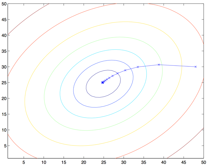
The ellipses in the figure are a contour plot of a quadratic function. Also shown is the trajectory produced by gradient descent, started at $(48,30)$. The $x$’s drawn in the figure (joined by straight lines) mark the values of $\theta$ that gradient descent passed through.
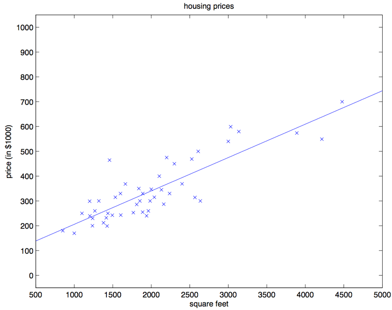
Running batch gradient descent on our earlier housing data set to fit $\theta$, and predicting house price as a function of living area, we obtain $\theta_0 = 71.27, \theta_1 = 0.1345$. If we plot $h_{\theta}(x)$ as a function of $x$, and also plot the existing data points in the training set, we get the following figure:
If the number of bedrooms is added to the data set as an input feature, the result is $\theta_0 = 89.60, \theta_1 = 0.1392, \theta_2 = -8.738$.
That result was obtained with batch gradient descent. There is another method that can replace batch gradient descent, and it also works well. It is as follows:
$$ \begin{aligned} &\qquad\text{Loop: }\{ \\ &\qquad\qquad \text{for }i\text{ from }1\text{ to }m,\{ \\ &\qquad\qquad\qquad\theta_j := \theta_j +\alpha(y^{(i)}-h_{\theta}(x^{(i)}))x_j^{(i)} \qquad(\text{for every }j) \\ &\qquad\qquad\} \\ &\qquad\} \end{aligned} $$In this algorithm we loop over the whole training set, and every time we encounter a training example we update the parameters according to the error gradient on that single example. This algorithm is called stochastic gradient descent, or incremental gradient descent. Batch gradient descent must scan the entire training set before it can take its first step. When the training set size $m$ becomes very large, the resulting cost is a poor tradeoff. Stochastic gradient descent does not have this problem: it can start immediately and operate on each example as it is encountered. Usually, stochastic gradient descent finds a $\theta$ sufficiently close to the minimum faster than batch gradient descent does. (Note also that it may never converge to the minimum, and $\theta$ may keep oscillating near the minimum of $J(\theta)$. In practice, however, most of those values near the minimum are already close enough to meet our accuracy requirements, so they are acceptable.)$^2$ For these reasons, especially when the training set is large, stochastic gradient descent is often preferred to batch gradient descent.
2 The more common situation is that we already have a description of the data set and a chosen learning rate $\alpha$, then run stochastic gradient descent while gradually letting the learning rate $\alpha$ tend to $0$ as the algorithm runs. That also guarantees that the parameters we finally obtain converge to the minimum, rather than oscillating around it. (Translator’s note: for all of the reasons above, stochastic gradient descent is usually recommended over batch gradient descent, especially when the training set is large.)
2 The Normal Equations
Gradient descent, as described above, is one way to find a minimum of $J$. Let us now look at another implementation. It is straightforward to derive, and it does not require an iterative algorithm. The idea is to find the minimum of $J$ directly by locating the $\theta_j$ at which the corresponding derivative is $0$. We want to do this without writing out a large pile of algebra or several pages of matrix calculus, so we first introduce some notation for matrix derivatives.
2.1 Matrix Derivatives
Suppose a function $f: R^{m\times n} \to R$ maps an $m\times n$ matrix to the real numbers. Then the derivative of $f$ with respect to a matrix $A$ is defined as:
$$ \nabla_A f(A)=\begin{bmatrix} \frac {\partial f}{\partial A_{11}} & \dots & \frac {\partial f}{\partial A_{1n}} \\ \vdots & \ddots & \vdots \\ \frac {\partial f}{\partial A_{m1}} & \dots & \frac {\partial f}{\partial A_{mn}} \\ \end{bmatrix} $$Thus the gradient $\nabla_A f(A)$ is itself an $m\times n$ matrix, whose $(i,j)$-th entry is $\frac {\partial f}{\partial A_{ij}}$.
Suppose $ A =\begin{bmatrix} A_{11} & A_{12} \\ A_{21} & A_{22} \\ \end{bmatrix} $ is a $2\times 2$ matrix, and the given function $f:R^{2\times 2} \to R$ is:
$$ f(A) = \frac 32A_{11}+5A^2_{12}+A_{21}A_{22} $$Here $A_{ij}$ means the $(i,j)$-th entry of the matrix $A$. The gradient is then:
$$ \nabla _A f(A) =\begin{bmatrix} \frac 32 & 10A_{12} \\ A_{22} & A_{21} \\ \end{bmatrix} $$We also introduce the trace operator, written $"tr"$. For a given $n\times n$ square matrix $A$, its trace is defined as the sum of the diagonal entries:
$$ trA = \sum^n_{i=1} A_{ii} $$If $a$ is a real number, then $a$ can in fact be viewed as a $1\times 1$ matrix, and the trace of $a$ is $tr a = a$. (If you have not seen this “operator notation” before, you can think of the trace of $A$ as $tr(A)$, or as a $trace$ function acting on the matrix $A$. It is more often written without parentheses.)
If two matrices $A$ and $B$ are such that $AB$ is square, the trace has a special property: $trAB = trBA$ (prove this yourself). From that one can deduce identities such as:
$$ trABC=trCAB=trBCA \\ trABCD=trDABC=trCDAB=trBCDA $$The following identities involving the trace are also easy to prove. Here $A$ and $B$ are square matrices, and $a$ is a real number:
$$ trA=trA^T \\ tr(A+B)=trA+trB \\ tr a A=a trA $$Next we state, without proof, some matrix derivatives (some of them are not needed until the end of this section). Note also that $A$ in equation $(4)$ must be a non-singular square matrix, and $|A|$ denotes the determinant of the matrix $A$. We then have the following identities:
$$ \begin{aligned} \nabla_A tr AB & = B^T & \text{(1)}\\ \nabla_{A^T} f(A) & = (\nabla_{A} f(A))^T &\text{(2)}\\ \nabla_A tr ABA^TC& = CAB+C^TAB^T &\text{(3)}\\ \nabla_A|A| & = |A|(A^{-1})^T &\text{(4)}\\ \end{aligned} $$To make our matrix-calculus notation more concrete, let us explain the first of these identities in detail. Suppose we have a fixed matrix $B \in R^{n\times m}$ (note the order: $n\times m$, meaning that the entries of $B$ are real and that $B$ is an $n\times m$ matrix). We can then define a function $f: R^{m\times n} \to R$ by $f(A) = trAB$. This matrix product is meaningful: if $A \in R^{m\times n}$, then $AB$ is square, and the trace applies to square matrices. Thus $f$ actually maps $R^{m\times n}$ to the real numbers $R$. We can then use matrix derivatives to find $\nabla_Af(A)$, and this derivative is itself an $m \times n$ matrix. Identity $(1)$ above says that the $(i,j)$-th entry of this derivative matrix equals the $(i,j)$-th entry of $B^T$ (the transpose of $B$), or, more directly, $B_{ji}$.
Identities $(1\text{-}3)$ are all straightforward, and their proofs are left as exercises. Identity $(4)$ is derived using the adjugate of the inverse matrix.$^3$
3 Suppose we define a matrix $A'$ whose $(i,j)$-th entry is $(-1)^{i+j}$ times the determinant of the matrix obtained by deleting row $i$ and column $j$ of $A$. One can prove that $A^{-1} = (A')^T /|A|$. (You can check this, for example, by seeing what $A^{-1}$ looks like when $A$ is a $2\times 2$ matrix, and then generalizing. If you want a proof of results of this kind, consult an intermediate or advanced linear algebra textbook, such as Charles Curtis, 1991, Linear Algebra, Springer.) This means $A' = |A|(A^{-1})^T$. Furthermore, the determinant of a matrix $A$ can also be written $|A| = \sum_j A_{ij}A'_{ij}$. Because $(A')_{ij}$ does not depend on $A_{ij}$ (as can be seen from the definition), this means $(\frac \partial {\partial A_{ij}})|A| = A'_{ij}$. Putting these facts together yields the result above.
2.2 Least Squares Revisited
With the matrix-derivative tool roughly in hand, we continue and use a closed-form solution to find the value of $\theta$ that minimizes $J(\theta)$. First we rewrite $J$ in matrix–vector notation.
Given a training set, define the design matrix $X$ to be an $m\times n$ matrix (in fact, if we account for the intercept term, the $\theta_0$ term, it should be an $m\times (n+1)$ matrix) that contains the input values of the training examples as its rows:
$$ X =\begin{bmatrix} -(x^{(1)}) ^T-\\ -(x^{(2)}) ^T-\\ \vdots \\ -(x^{(m)}) ^T-\\ \end{bmatrix} $$Next, let $\vec{y}$ be an $m$-dimensional vector containing all the target values in the training set:
$$ y =\begin{bmatrix} y^{(1)}\\ y^{(2)}\\ \vdots \\ y^{(m)}\\ \end{bmatrix} $$Because $h_\theta (x^{(i)}) = (x^{(i)})^T\theta$ (Translator’s note: I have not yet tried to derive this; at a glance it does not look hard), one can show that the following equality holds:
$$ \begin{aligned} X\theta - \vec{y} &= \begin{bmatrix} (x^{(1)})^T\theta \\ \vdots \\ (x^{(m)})^T\theta\\ \end{bmatrix} - \begin{bmatrix} y^{(1)}\\ \vdots \\ y^{(m)}\\ \end{bmatrix}\\ & = \begin{bmatrix} h_\theta (x^{1}) -y^{(1)}\\ \vdots \\ h_\theta (x^{m})-y^{(m)}\\ \end{bmatrix}\\ \end{aligned} $$For a vector $\vec{z}$, we have $z^T z = \sum_i z_i^2$. Using this property, one can derive:
$$ \begin{aligned} \frac 12(X\theta - \vec{y})^T (X\theta - \vec{y}) &=\frac 12 \sum^m_{i=1}(h_\theta (x^{(i)})-y^{(i)})^2\\ &= J(\theta) \end{aligned} $$Finally, to minimize $J$, find the derivative of this function with respect to $\theta$. Combining identities $(2)$ and $(3)$, we obtain the following identity $(5)$:
$$ \nabla_{A^T} trABA^TC =B^TA^TC^T+BA^TC \qquad \text{(5)} $$Therefore:
$$ \begin{aligned} \nabla_\theta J(\theta) &= \nabla_\theta \frac 12 (X\theta - \vec{y})^T (X\theta - \vec{y}) \\ &= \frac 12 \nabla_\theta (\theta ^TX^TX\theta -\theta^T X^T \vec{y} - \vec{y} ^TX\theta +\vec{y}^T \vec{y})\\ &= \frac 12 \nabla_\theta tr(\theta ^TX^TX\theta -\theta^T X^T \vec{y} - \vec{y} ^TX\theta +\vec{y}^T \vec{y})\\ &= \frac 12 \nabla_\theta (tr \theta ^TX^TX\theta - 2tr\vec{y} ^T X\theta)\\ &= \frac 12 (X^TX\theta+X^TX\theta-2X^T\vec{y}) \\ &= X^TX\theta-X^T\vec{y}\\ \end{aligned} $$In the third step we used the fact that the trace of a real number is the real number itself. In the fourth step we used $trA = trA^T$. In the fifth step we used identity $(5)$, with $A^T =\theta, B=B^T =X^TX, C=I$, and we also used identity $(1)$. To minimize $J$, set the derivative equal to $0$. That yields the normal equations:
$$ X^TX\theta =X^T\vec{y} $$So the $\theta$ that minimizes $J(\theta)$ is
$$ \theta = (X^TX)^{-1}X^T\vec{y} $$3 Probabilistic Interpretation
When facing a regression problem, one may ask why we choose linear regression, and in particular why we choose least squares as the cost function $J$. In this section we give a set of basic probabilistic assumptions under which least-squares regression emerges as a very natural algorithm.
First assume that the target variables and the inputs are related by:
$$ y^{(i)}=\theta^T x^{(i)}+ \epsilon ^{(i)} $$Here $\epsilon^{(i)}$ is an error term. It captures the effect of variables left out of the model (for example, some features may clearly affect house prices, but we ignored them when doing the regression) or random noise. Assume further that the $\epsilon^{(i)}$ are independently and identically distributed (IID), following a Gaussian distribution (also called a normal distribution) with mean $0$ and variance $\sigma^2$. We can write this assumption as $\epsilon^{(i)} \sim N(0, \sigma^2)$. The density of $\epsilon^{(i)}$ is then:
$$ p(\epsilon ^{(i)} )= \frac 1{\sqrt{2\pi}\sigma} exp (- \frac {(\epsilon ^{(i)} )^2}{2\sigma^2}) $$This implies the following equality:
$$ p(y ^{(i)} |x^{(i)}; \theta)= \frac 1{\sqrt{2\pi}\sigma} exp (- \frac {(y^{(i)} -\theta^T x ^{(i)} )^2}{2\sigma^2}) $$The notation $"p(y ^{(i)} |x^{(i)}; \theta)"$ means that this is the distribution of $y^{(i)}$ given $x^{(i)}$, with $\theta$ standing for the parameters of that distribution. Note that we should not condition on $\theta$, as in $"p(y ^{(i)} |x^{(i)},\theta)"$, because $\theta$ is not a random variable. The distribution of $y^{(i)}$ can also be written $y^{(i)} | x^{(i)}; \theta \sim N(\theta ^T x^{(i)}, \sigma^2)$.
Given a design matrix $X$ that contains all the $x^{(i)}$, and given $\theta$, what is the distribution of the $y^{(i)}$? The probability of the data is given in the form $p(\vec{y}|X;\theta)$. For a fixed value of $\theta$, this quantity can usually be viewed as a function of $\vec{y}$ (and it can also be viewed as a function of $X$). When we want to treat it as a function of $\theta$, we call it the likelihood function:
$$ L(\theta) =L(\theta;X,\vec{y})=p(\vec{y}|X;\theta) $$Combining this with the earlier independence assumption on the $\epsilon^{(i)}$ (and making the same assumption for the $y^{(i)}$ given the $x^{(i)}$), we can rewrite the equality above as:
$$ \begin{aligned} L(\theta) &=\prod ^m _{i=1}p(y^{(i)}|x^{(i)};\theta)\\ &=\prod ^m _{i=1} \frac 1{\sqrt{2\pi}\sigma} exp(- \frac {(y^{(i)}-\theta^T x^{(i)})^2}{2\sigma^2})\\ \end{aligned} $$Now that we have a probabilistic model of the relationship between $y^{(i)}$ and $x^{(i)}$, how should we choose our best guess of the parameter $\theta$? The method of maximum likelihood tells us to choose the $\theta$ that makes the likelihood of the data as large as possible. That is, the $\theta$ we want is one that maximizes the function $L(\theta)$.
Besides maximizing $L(\theta)$, we may maximize any strictly increasing function of $L(\theta)$. If, instead of using $L(\theta)$ directly, we use the logarithm and maximize the log likelihood $l(\theta)$, differentiation becomes a bit simpler:
$$ \begin{aligned} l(\theta) &=\log L(\theta)\\ &=\log \prod ^m _{i=1} \frac 1{\sqrt{2\pi}\sigma} exp(- \frac {(y^{(i)}-\theta^T x^{(i)})^2}{2\sigma^2})\\ &= \sum ^m _{i=1}log \frac 1{\sqrt{2\pi}\sigma} exp(- \frac {(y^{(i)}-\theta^T x^{(i)})^2}{2\sigma^2})\\ &= m \log \frac 1{\sqrt{2\pi}\sigma}- \frac 1{\sigma^2}\cdot \frac 12 \sum^m_{i=1} (y^{(i)}-\theta^Tx^{(i)})^2\\ \end{aligned} $$Therefore, maximizing $l(\theta)$ means minimizing the following expression:
$$ \frac 12 \sum^m _{i=1} (y^{(i)}-\theta^Tx^{(i)})^2 $$We can see that this expression is exactly $J(\theta)$, the original least-squares cost function.
To summarize: under our probabilistic assumptions on the data, the $\theta$ obtained by least-squares regression is the same as the $\theta$ estimated by maximum likelihood. This is a set of assumptions under which least-squares regression can be judged a very natural method, precisely because it performs maximum likelihood estimation. (Note that these probabilistic assumptions are not necessary in order to justify least squares as a sound and reasonable procedure, and there may be — and indeed are — other natural assumptions under which least squares can be assessed.)
Note also that, in the discussion above, our final choice of $\theta$ does not depend on $\sigma^2$, and indeed we found the result without knowing $\sigma^2$. We will make use of this fact later, when we discuss the exponential family and generalized linear models.
4 Locally Weighted Linear Regression
Suppose the problem is still to predict $y$ from an $x \in R$ that takes values in the real numbers. The figure at the lower left shows a fit of $y = \theta_0 + \theta_1 x$ to a data set. We can clearly see that the trend in the data is not a strict straight line, so a straight-line fit is not a good method.
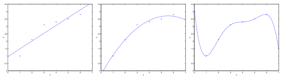
This time, instead of a straight line, add a quadratic term and fit $y = \theta_0 + \theta_1 x + \theta_2 x^2$. (See the middle figure.) Clearly, the more features we add, the better the fit. Adding too many features, however, is also dangerous: the rightmost figure uses a fifth-degree polynomial $y = \sum^5_{j=0} \theta_j x^j$. The figure shows that, although the fitted curve passes perfectly through every point in the current data set, we obviously cannot regard this curve as a suitable tool for prediction, for example for predicting house price $y$ from a different living area $x$. Setting aside the formal definitions of these terms, let us simply say that the leftmost picture is an example of underfitting: one can clearly see that the fitted model has missed structure in the data set. The rightmost picture is an example of overfitting. (Later in this course, when we discuss learning theory, we will give the standard definitions of these concepts, and also discuss what goodness of fit means as a test of how good a hypothesis is.)
As mentioned earlier, and as this example shows, feature choice is very important if a learning algorithm is to work well. (When we get to model selection, we will also see algorithms that can automatically choose a good set of features.) In this section we briefly discuss locally weighted linear regression (abbreviated LWR). The method assumes that there is enough training data, and it down-weights features that are less important. The discussion here will be fairly brief, because the homework asks students to explore the various properties of the LWR algorithm themselves.
In the original version of linear regression, predicting at a query point $x$ — that is, evaluating $h(x)$ — goes through the following steps:
- Fit the parameters $\theta$ so as to minimize the sum of squared differences between the values in the data set and the fitted values, $\sum_i(y^{(i)} - \theta^T x^{(i)} )^2$ (the idea of least squares);
- Output $\theta^T x$.
Correspondingly, the steps of locally weighted linear regression (LWR) are:
- Fit the parameters $\theta$ so as to minimize the weighted distance $\sum_i w^{(i)}(y^{(i)} - \theta^T x^{(i)} )^2$;
- Output $\theta^T x$.
The $w^{(i)}$ in the expression above are nonnegative weights. Intuitively, if the weight $w^{(i)}$ for some $i$ is especially large, then when choosing the fitted parameters $\theta$ we should try hard to make $(y^{(i)} - \theta^T x^{(i)} )^2$ small at that point. If the weight $w^{(i)}$ is especially small, then the corresponding $(y^{(i)} - \theta^T x^{(i)} )^2$ is essentially ignored during the fit.
A fairly standard formula for choosing the weights is:$^4$
$$ w^{(i)} = exp(- \frac {(x^{(i)}-x)^2}{2\tau^2}) $$4 If $x$ is a vector with values, the formula above must be generalized, giving $w^{(i)} = exp(- \frac {(x^{(i)}-x)^T(x^{(i)}-x)}{2\tau^2})$, or $w^{(i)} = exp(- \frac {(x^{(i)}-x)^T\Sigma ^{-1}(x^{(i)}-x)}{2})$, depending on whether one chooses to use $\tau$ or $\Sigma$.
Note that the weights depend on the particular point $x$, and those points are exactly the points at which we want to make a prediction. Furthermore, if $|x^{(i)} - x|$ is very small, then the weight $w^{(i)}$ is close to $1$; conversely, if $|x^{(i)} - x|$ is very large, then the weight $w^{(i)}$ becomes small. So, in the process of choosing $\theta$, training examples near the query point $x$ receive a much higher weight. ($\theta$ is chosen giving a much higher “weight” to the (errors on) training examples close to the query point $x$.) (Note also that, although the form of the weight equation is quite close to the density of a Gaussian distribution, the weights have no direct connection with the Gaussian distribution, especially since the weights are not random values and are not distributed as a normal or any other distribution.) As the distance from the point $x^{(i)}$ to the query point $x$ decreases, the weight of the training example also decreases, and the parameter $\tau$ controls the speed of that decrease. $\tau$ is also called the bandwidth parameter, and it is a parameter you will need to experience and experiment with in the homework.
Locally weighted linear regression is the first non-parametric algorithm we have encountered. The unweighted linear regression algorithm we saw earlier is a parametric learning algorithm, because it has a fixed, finite number of parameters (the $\theta_i$) that are used to fit the data. Once we have fit the $\theta_i$, we store them, and we no longer need to keep the training examples in order to make further predictions. By contrast, if we use locally weighted linear regression, we must keep the entire training set around. The term “non-parametric” in a non-parametric algorithm roughly means that, in order to represent the hypothesis $h$ as growing linearly with the size of the data set, we need to store an amount of data that grows in a corresponding way. (The term “non-parametric” (roughly) refers to the fact that the amount of stuff we need to keep in order to represent the hypothesis $h$ grows linearly with the size of the training set.)
Part II: Classification and Logistic Regression
Next we turn to classification. A classification problem is actually much like a regression problem, except that the value of $y$ we now want to predict is restricted to a small number of discrete values. For the moment we focus on binary classification, meaning that the $y$ we need to decide takes only two values, $0$ or $1$. (Most of what we say here can also be extended to the multi-class case.) For example, if we want to build a spam filter, we can let $x^{(i)}$ denote some features of an email, and set $y$ to $1$ if the email is spam and $y$ to $0$ otherwise. $0$ may also be called the negative class, and $1$ the positive class; sometimes they are written “-” and “+” respectively. For a given $x^{(i)}$, the corresponding $y^{(i)}$ is also called the label of the training example.
5 Logistic Regression
We could of course still use the earlier linear regression algorithm to predict $y$ from a given $x$, simply ignoring the fact that $y$ is discrete. Examples built that way, however, easily run into trouble: the method is very inefficient and performs very poorly. And intuitively, a value of $h_\theta(x)$ greater than $1$ or less than $0$ is meaningless, because we have already established that $y \in \{0, 1\}$, so $y$ must be one of the two values $0$ and $1$.
So let us change the form of the hypothesis $h_\theta(x)$ to fix this problem. For example, we can choose the following function:
$$ h_\theta(x) = g(\theta^T x) = \frac 1{1+e^{-\theta^Tx}} $$where
$$ g(z)= \frac 1 {1+e^{-z}} $$This function is called the logistic function, or the sigmoid function. The figure below is the graph of $g(z)$:
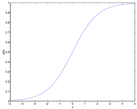
Notice that as $z\to +\infty$, $g(z)$ tends to $1$, and as $z\to -\infty$, $g(z)$ tends to $0$. Moreover, this $g(z)$, and hence $h(x)$, always stays between $0$ and $1$. We still set $x_0 = 1$ as at the beginning, so that $\theta^T x =\theta_0 +\sum^n_{j=1}\theta_jx_j$.
We now take $g$ as our chosen function. Other functions that increase smoothly from $0$ to $1$ could also be used, but later we will see some reasons for choosing $g$ (when we discuss generalized linear models, GLMs, and also generative learning algorithms). The choice of this logistic function is a natural one. Before going further, here are some properties of the derivative of the sigmoid function, that is, of $g'$:
$$ \begin{aligned} g'(z) & = \frac d{dz}\frac 1{1+e^{-z}}\\ & = \frac 1{(1+e^{-z})^2}(e^{-z})\\ & = \frac 1{(1+e^{-z})} \cdot (1- \frac 1{(1+e^{-z})})\\ & = g(z)(1-g(z))\\ \end{aligned} $$Given the logistic regression model, how do we fit a suitable $\theta$? We have already seen that, under a set of assumptions, least-squares regression can be derived from maximum likelihood estimation. Let us now make a set of statistical assumptions for this classification model, and then fit the parameters by maximum likelihood.
First assume:
$$ \begin{aligned} P(y=1|x;\theta)&=h_{\theta}(x)\\ P(y=0|x;\theta)&=1- h_{\theta}(x)\\ \end{aligned} $$A more compact way to write this is:
$$ p(y|x;\theta)=(h_\theta (x))^y(1- h_\theta (x))^{1-y} $$Assuming that the $m$ training examples were generated independently of one another, we can write the likelihood of the parameters as follows:
$$ \begin{aligned} L(\theta) &= p(\vec{y}| X; \theta)\\ &= \prod^m_{i=1} p(y^{(i)}| x^{(i)}; \theta)\\ &= \prod^m_{i=1} (h_\theta (x^{(i)}))^{y^{(i)}}(1-h_\theta (x^{(i)}))^{1-y^{(i)}} \\ \end{aligned} $$As before, taking the logarithm makes it easier to compute the maximum:
$$ \begin{aligned} l(\theta) &=\log L(\theta) \\ &= \sum^m_{i=1} y^{(i)} \log h(x^{(i)})+(1-y^{(i)})\log (1-h(x^{(i)})) \end{aligned} $$How do we maximize the likelihood? Much as we used derivatives for linear regression, this time we use gradient ascent. Written in vector form, the update is $\theta := \theta +\alpha \nabla _\theta l(\theta)$. (Note that the update equation uses a plus sign rather than a minus sign, because we are now looking for a maximum of a function rather than a minimum.) Again we start from a single training example $(x,y)$, take derivatives, and derive the stochastic gradient ascent rule:
In the derivation above we used the differentiation rule $g'(z)= g(z)(1-g(z))$. We then obtain the stochastic gradient ascent rule:
$$ \theta_j := \theta_j + \alpha (y^{(i)}-h_\theta (x^{(i)}))x_j^{(i)} $$If we compare this with the earlier LMS update rule, it looks quite similar. It is not the same algorithm, however, because $h_\theta(x^{(i)})$ is now defined to be a nonlinear function of $\theta^Tx^{(i)}$. Even so, it is a little surprising that we used different algorithms on different learning problems and arrived at update rules that look the same. Is this a coincidence, or is there a deeper reason behind it? We will get the answer when we study generalized linear models (GLMs). (See also the extra credit part of Q3 in Problem Set 1.)
6 Digression: The Perceptron Learning Algorithm
Let us briefly change the subject and talk about an algorithm with an interesting history, one that we will return to when we discuss learning theory. Imagine modifying logistic regression so as to “force” its output to be either $0$ or $1$. To do that, it is natural to change the definition of $g$ to a threshold function:
$$ g(z)= \begin{cases} 1 & if\quad z \geq 0 \\ 0 & if\quad z < 0 \end{cases} $$If, as before, we set $h_\theta(x) = g(\theta^T x)$, but use the threshold function above as the definition of $g$, and if we use the following update rule:
$$ \theta_j := \theta_j +\alpha(y^{(i)}-h_\theta (x^{(i)}))x_j^{(i)} $$then we obtain the perceptron learning algorithm.
In the 1960s, this “perceptron” was regarded as a rough model of how a single neuron in the brain works. Because the algorithm is so simple, it is also our starting point later in this course when we discuss learning theory. But note carefully: although the perceptron learning algorithm may look superficially similar to the other algorithms we have discussed, it is in fact an algorithm of an entirely different kind from logistic regression and least-squares linear regression. In particular, it is hard to give the perceptron’s predictions a meaningful probabilistic interpretation, and it is hard to derive the perceptron learning algorithm as a maximum likelihood estimation algorithm.
7 Another Algorithm for Maximizing $l(\theta)$
Returning to logistic regression with the sigmoid function $g(z)$, let us discuss another algorithm for maximizing $l(\theta)$.
Before we start, consider Newton’s method for finding a zero of an equation. Suppose we have a function $f:R \to R$ from the reals to the reals, and we want to find a $\theta$ satisfying $f(\theta)=0$, where $\theta\in R$ is a real number. Newton’s method updates $\theta$ as follows:
$$ \theta := \theta - \frac {f(\theta)}{f'(\theta)} $$There is a very natural interpretation of this method. We can think of it as approximating the function $f$ by a linear function: the line is the tangent to $f$, the current guess is $\theta$, and the way we solve is to find the point where the linear equation equals zero, take that zero as the next guess for $\theta$, and repeat.
Here is an illustration of Newton’s method:
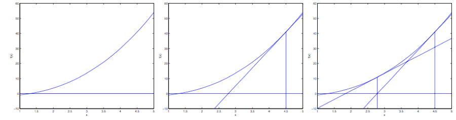
In the leftmost figure, the function $f$ is shown together with the line $y=0$. We want a $\theta$ such that $f(\theta)=0$. That value of $\theta$ is about $1.3$. Suppose our initial guess is set to $\theta=4.5$. Newton’s method draws a tangent line at $\theta=4.5$ (the middle figure). That gives the location of the next guess for $\theta$, namely the zero of this tangent, about $2.8$. The rightmost figure shows the result of running the iteration once more, at which point $\theta$ is about $1.8$. After a few iterations like this, we quickly approach $\theta=1.3$.
Newton’s method is a way to solve $f(\theta) = 0$. Can we use it to maximize the function $l$? The maximum of $l$ should correspond to a point where its derivative $l'(\theta)$ equals zero. So, by setting $f(\theta) = l'(\theta)$, we can likewise use Newton’s method to find the maximum of $l$, and we obtain the following update rule:
$$ \theta := \theta - \frac {l'(\theta)}{l''(\theta)} $$(As a further exercise, think about this: if we want to use Newton’s method to find a minimum of a function rather than a maximum, how should we modify it?) (Translator's note: try the zero of the normal line.)
Finally, in our logistic regression setting, $\theta$ is a vector of values, so we need to extend Newton’s method to this case. Newton’s method extended to several dimensions, also called the Newton–Raphson method, is as follows:
$$ \theta := \theta - H^{-1}\nabla_\theta l(\theta) $$Here $\nabla_\theta l(\theta)$ is, as in the earlier examples, the vector of partial derivatives of $l(\theta)$ with respect to the $\theta_i$. And $H$ is an $n\times n$ matrix — in fact, if the intercept term is included, it should be $(n + 1)\times (n + 1)$ — called the Hessian. Its detailed definition is:
$$ H_{ij}= \frac {\partial^2 l(\theta)}{\partial \theta_i \partial \theta_j} $$Newton’s method usually converges faster than (batch) gradient descent, and it reaches the minimum in far fewer iterations. A single iteration of Newton’s method, however, often costs more than one step of gradient descent, because one must find and invert an $n\times n$ Hessian matrix. As long as this $n$ is not too large, Newton’s method is usually still faster. When Newton’s method is used to maximize the likelihood $l(\theta)$ in logistic regression, the resulting method is also called Fisher scoring.
Part III: Generalized Linear Models$^5$
5 The material presented in this section was inspired by the following two works: Michael I. Jordan, Learning in graphical models (unpublished book draft), and McCullagh and Nelder, Generalized Linear Models (2nd ed.).
So far we have seen a regression example and a classification example. In the regression example, the distribution we obtained was $y|x; \theta \sim N(\mu, \sigma^2)$. In the classification example, it was $y|x; \theta \sim Bernoulli(\phi)$, where $\mu$ and $\phi$ are each some function of $x$ and $\theta$. In this section we will see that both methods are special cases of a more broadly used model, called a generalized linear model. We will also discuss how other models in the generalized linear model family are derived, and how they are applied to other classification and regression problems.
8 The Exponential Family
Before studying GLMs, we need to define exponential family distributions. We say that a distribution belongs to the exponential family if it can be written in the following form:
$$ p(y;\eta) =b(y)exp(\eta^TT(y)-a(\eta)) \qquad \text{(6)} $$In the expression above, $\eta$ is called the natural parameter of the distribution (also called the canonical parameter). $T(y)$ is called the sufficient statistic; for the distributions we use here, usually $T(y) = y$. And $a(\eta)$ is the log partition function. The quantity $e^{-a(\eta)}$ essentially plays the role of a normalization constant, that is, it ensures that the sum or integral of $p(y; \eta)$ equals $1$.
Given $T$, $a$, and $b$, one defines a family (or set) of distributions parameterized by $\eta$. By varying $\eta$, we obtain different distributions in this family.
The Bernoulli and Gaussian distributions we are looking at now both belong to the exponential family. The Bernoulli distribution has mean $\phi$, also written $Bernoulli(\phi)$, and the specified distribution is over $y \in \{0, 1\}$, so $p(y = 1; \phi) = \phi$ and $p(y = 0;\phi) = 1-\phi$. Changing $\phi$ then yields a family of Bernoulli distributions with different means. The Bernoulli distributions obtained by varying $\phi$, as we now show, belong to the exponential family. That is, given a choice of $T$, $a$, and $b$, equation $(6)$ above can be used to specify a particular Bernoulli distribution.
We write the Bernoulli distribution as follows:
$$ \begin{aligned} p(y;\phi) & = \phi ^y(1-\phi)^{1-y}\\ & = exp(y \log \phi + (1-y)\log(1-\phi))\\ & = exp( (log (\frac {\phi}{1-\phi}))y+\log (1-\phi) )\\ \end{aligned} $$The natural parameter is therefore given by $\eta = log (\frac \phi {1 - \phi})$. Interestingly, if we invert this definition and solve for $\phi$ in terms of $\eta$, we get $\phi = 1/ (1 + e^{-\eta})$. This is exactly the sigmoid function we just saw! When we treat logistic regression as a generalized linear model (GLM), we will also obtain:
$$ \begin{aligned} T(y) &= y \\ a( \eta) & = - \log (1- \phi) \\ & = \log {(1+ e^ \eta)}\\ b(y)&=1 \end{aligned} $$The equations above show that the Bernoulli distribution can be written in the form of equation $(6)$, using a suitable choice of $T$, $a$, and $b$.
Next, consider the Gaussian distribution. Recall that, when we derived linear regression, the value of $\sigma^2$ had no effect on our final choice of $\theta$ or on $h_\theta(x)$. So we may assign $\sigma^2$ any value we like. To simplify the derivation, set $\sigma^2 = 1$.$^6$ We then have:
$$ \begin{aligned} p(y;\mu) &= \frac 1{\sqrt{2\pi}} exp (- \frac 12 (y-\mu)^2) \\ & = \frac 1{\sqrt{2\pi}} exp (- \frac 12 y^2) \cdot exp (\mu y -\frac 12 \mu^2) \\ \end{aligned} $$6 If we leave $\sigma^2$ as a variable, the Gaussian distribution can also be written in exponential-family form, where $\eta \in R^2$ is a two-dimensional vector depending on both $\mu$ and $\sigma$. For the purposes of generalized linear models (GLMs), however, the parameter $\sigma^2$ can also be viewed through a more general definition of the exponential family: $p(y; \eta, \tau ) = b(a, \tau ) exp((\eta^T T (y) - a(\eta))/c(\tau))$. Here $\tau$ is called the dispersion parameter. For the Gaussian distribution, $c(\tau) = \sigma^2$. We have already simplified the discussion above, so for the cases we need to consider we do not need this more general definition.
We can thus see that the Gaussian distribution belongs to the exponential family, and it can be written as follows:
$$ \begin{aligned} \eta & = \mu \\ T(y) & = y \\ a(\eta) & = \mu ^2 /2\\ & = \eta ^2 /2\\ b(y) & = (1/ \sqrt {2\pi })exp(-y^2/2) \end{aligned} $$There are many other distributions in the exponential family:
- for example, the multinomial distribution, which we will see shortly;
- the Poisson distribution, used to model count data, which will also appear later in the problem sets;
- the gamma and the exponential distributions, used to model continuous, nonnegative random variables, such as time intervals;
- the beta and the Dirichlet distributions, which are distributions over probabilities;
- and many others, which we will not list one by one.
In the next section we discuss a more general “recipe” for modeling, in which $y$ (given $x$ and $\theta$) may follow any of the distributions above.
9 Constructing GLMs
Suppose you want to build a model to estimate the number of customers who come to your store in a given hour (or the number of page views on your website), based on certain features $x$, such as the store’s promotions, recent advertising, the weather, the day of the week, and so on. We already know that the Poisson distribution is usually a good fit for modeling visitor counts. Knowing that, how do we build a model for this particular problem? Fortunately, the Poisson distribution is a member of the exponential family, so we can apply a generalized linear model (GLM) to the problem. In this section we describe a method for constructing a generalized linear model for problems of the kind just mentioned.
More generally, consider a classification or regression problem in which we want to predict the value of some random variable $y$ as a function of $x$. To derive a generalized linear model appropriate to this problem, we make the following three assumptions about our model, that is, about the conditional distribution of $y$ given $x$:
- $y | x; \theta \sim Exponential Family(\eta)$. That is, given $x$ and $\theta$, the distribution of $y$ belongs to the exponential family and is an exponential-family distribution with parameter $\eta$. — Assumption 1
- Given $x$, the goal is to predict the expected value of $T(y)$ corresponding to this given $x$. In the great majority of our examples, $T(y) = y$, which means that the prediction $h(x)$ output by our learning hypothesis $h$ should satisfy $h(x) = E[y|x]$. (Note that this assumption is satisfied by the choice of $h_\theta(x)$ in both logistic regression and linear regression. For example, in logistic regression, $h_\theta (x) = [p (y = 1|x; \theta)] =[ 0 \cdot p (y = 0|x; \theta)+1\cdot p(y = 1|x;\theta)] = E[y|x;\theta]$. Translator’s note: $E[y|x]$ here should mean the expected value of $y$ given $x$.) — Assumption 2
- The natural parameter $\eta$ and the input $x$ are linearly related: $\eta = \theta^T x$, or, if $\eta$ is a vector of values, $\eta_i = \theta_i^T x$. — Assumption 3
Of the assumptions above, the third may look the least well justified, so it is more appropriate to regard this third assumption as a design choice we make when designing generalized linear models, rather than as an assumption. These three assumptions, or design choices, can then be used to derive a very suitable class of learning algorithms, namely generalized linear models (GLMs). This class of models has many particularly friendly and desirable properties; for example, they are easy to learn. Moreover, models of this kind are usually very effective for modeling different types of distributions on $y$. Below, for example, we will briefly show how both logistic regression and ordinary least squares can be derived as generalized linear models.
9.1 Ordinary Least Squares
What we discuss in this section is that ordinary least squares is in fact a special case of a generalized linear model. Consider the following setting. The target variable $y$ (also called the response variable in GLM terminology) is continuous, and we model the distribution of $y$ given $x$ as a Gaussian distribution $N(\mu, \sigma^2)$, where $\mu$ may be a function of $x$. In this way we make the $ExponentialFamily(\eta)$ distribution above into a Gaussian distribution. Earlier we noted that, when the Gaussian distribution is written as an exponential-family distribution, $\mu = \eta$. We therefore obtain:
$$ \begin{aligned} h_\theta(x)& = E[y|x;\theta] \\ & = \mu \\ & = \eta \\ & = \theta^Tx\\ \end{aligned} $$The first line is based on Assumption 2. The second equality is based on the fact that if $y|x; \theta \sim N(\mu, \sigma^2)$, then the expectation of $y$ is $\mu$. The third equality is based on Assumption 1, together with the property $\mu = \eta$ that we derived earlier when writing the Gaussian distribution as an exponential-family distribution. The last equality is based on Assumption 3.
9.2 Logistic Regression
Next let us look again at logistic regression. Here we are still considering a binary classification problem, that is, $y \in \{0, 1\}$. Given that $y$ is a value chosen from two possibilities, it is natural to choose the Bernoulli distribution to model the distribution of $y$ given $x$. When we wrote the Bernoulli distribution as an exponential-family distribution, we had $\phi = 1/ (1 + e^{-\eta})$. Note also that if $y|x; \theta \sim Bernoulli(\phi)$, then $E[y|x; \theta] = \phi$. So, by a derivation similar to the one we just gave for ordinary least squares, we have:
$$ \begin{aligned} h_\theta(x)& = E[y|x;\theta] \\ & = \phi \\ & = 1/(1+ e^{-\eta}) \\ & = 1/(1+ e^{-\theta^Tx})\\ \end{aligned} $$The equality above therefore gives the form of the hypothesis: $h_\theta(x) = 1/ (1 + e^{-\theta^T x})$. If you previously wondered how we came up with $1/ (1 + e^{-z})$ as the function for logistic regression, this is one answer: once we assume that the distribution of $y$ conditional on $x$ is Bernoulli, the definitions of generalized linear models and of the exponential family yield this expression.
A bit more terminology. The function $g$ that gives the mean of the distribution, as a function of the natural parameter, $g(\eta) = E[T(y); \eta]$, is called the canonical response function, and its inverse $g^{-1}$ is called the canonical link function. Thus, for the Gaussian distribution, the canonical response function is exactly the identity function; for the Bernoulli distribution, the canonical response function is the logistic function.$^7$
7 Many textbooks use $g$ for the link function and the inverse $g^{-1}$ for the response function. We do the reverse. This follows an early usage in machine learning, and using it this way connects more smoothly with the other courses that follow.
9.3 Softmax Regression
Let us look at one more example of a generalized linear model. Consider a classification problem in which the response variable $y$ can take any one of $k$ values, that is, $y \in \{1, 2, \ldots, k\}$. For example, the classification we want to do this time is more complicated than a binary split of email into spam and non-spam. We might want three classes, such as spam, personal mail, and work-related mail. The response variable is still discrete, but it no longer takes only two values. We therefore model it with the multinomial distribution.
We now derive a generalized linear model from this multinomial distribution. To do that, we first describe the multinomial distribution itself as an exponential-family distribution.
To parameterize a multinomial that can have $k$ different output values, one can use $k$ parameters $\phi_1,\ldots,\phi_k$, corresponding to the probabilities of the respective outputs. That many parameters may be too many, and the form is also cumbersome. They are not necessarily mutually independent either (for any one of the $\phi_i$, once the other $k-1$ values are known, the last one is determined, because the total equals $1$, that is, $\sum^k_{i=1} \phi_i = 1$). So we drop one parameter and parameterize the multinomial with only $k-1$ parameters, $\phi_1,\ldots,\phi_{k-1}$, where $\phi_i = p(y = i; \phi)$ and $p(y = k; \phi) = 1 - \sum^{k-1}_{i=1}\phi_i$. For ease of presentation we also set $\phi_k = 1 - \sum_{i=1}^{k-1} \phi_i$, but note carefully that this is not a parameter. It is completely determined by the other $k-1$ parameters.
To express a multinomial as an exponential-family distribution, we also define $T(y) \in R^{k-1}$ as follows:
$$ T(1)= \begin{bmatrix} 1\\ 0\\ 0\\ \vdots \\ 0\\ \end{bmatrix}, T(2)= \begin{bmatrix} 0\\ 1\\ 0\\ \vdots \\ 0\\ \end{bmatrix}, T(3)= \begin{bmatrix} 0\\ 0\\ 1\\ \vdots \\ 0\\ \end{bmatrix}, T(k-1)= \begin{bmatrix} 0\\ 0\\ 0\\ \vdots \\ 1\\ \end{bmatrix}, T(k)= \begin{bmatrix} 0\\ 0\\ 0\\ \vdots \\ 0\\ \end{bmatrix}, $$This time, unlike the earlier examples, we no longer have $T(y) = y$. Also, $T(y)$ is now a $(k-1)$-dimensional vector rather than a real number. The $i$-th element of the vector $T(y)$ is written $(T(y))_i$.
We now introduce a very useful piece of notation. The indicator function $1\{\cdot\}$ equals $1$ if its argument is true and $0$ otherwise ($1\{True\} = 1, 1\{False\} = 0$). For example, $1\{2 = 3\} = 0$, while $1\{3 = 5 - 2\} = 1$. So we can write the relationship between $T(y)$ and $y$ as $(T(y))_i = 1\{y = i\}$. (Before reading on, make sure you understand that this expression is true!) On that basis, we have $E[(T(y))_i] = P(y = i) = \phi_i$.
Everything is now in place to write the multinomial as an exponential-family distribution. It is as follows:
$$ \begin{aligned} p(y;\phi) &=\phi_1^{1\{y=1\}}\phi_2^{1\{y=2\}}\dots \phi_k^{1\{y=k\}} \\ &=\phi_1^{1\{y=1\}}\phi_2^{1\{y=2\}}\dots \phi_k^{1-\sum_{i=1}^{k-1}1\{y=i\}} \\ &=\phi_1^{(T(y))_1}\phi_2^{(T(y))_2}\dots \phi_k^{1-\sum_{i=1}^{k-1}(T(y))_i } \\ &=exp((T(y))_1 log(\phi_1)+(T(y))_2 log(\phi_2)+\dots+(1-\sum_{i=1}^{k-1}(T(y))_i)log(\phi_k)) \\ &= exp((T(y))_1 log(\frac{\phi_1}{\phi_k})+(T(y))_2 log(\frac{\phi_2}{\phi_k})+\dots+(T(y))_{k-1}log(\frac{\phi_{k-1}}{\phi_k})+log(\phi_k)) \\ &=b(y)exp(\eta^T T(y)-a(\eta)) \end{aligned} $$where
$$ \begin{aligned} \eta &= \begin{bmatrix} \log (\phi _1/\phi _k)\\ \log (\phi _2/\phi _k)\\ \vdots \\ \log (\phi _{k-1}/\phi _k)\\ \end{bmatrix}, \\ a(\eta) &= -\log (\phi _k)\\ b(y) &= 1\\ \end{aligned} $$In this way we have written the multinomial as an exponential-family distribution.
The link function corresponding to $i$ (for $i = 1, \ldots, k$) is:
$$ \eta_i =\log \frac {\phi_i}{\phi_k} $$For convenience, we also define $\eta_k = \log (\phi_k/\phi_k) = 0$. Taking the inverse of the link function and thereby deriving the response function, we obtain:
$$ \begin{aligned} e^{\eta_i} &= \frac {\phi_i}{\phi_k}\\ \phi_k e^{\eta_i} &= \phi_i \qquad\text{(7)}\\ \phi_k \sum^k_{i=1} e^{\eta_i}&= \sum^k_{i=1}\phi_i= 1\\ \end{aligned} $$This shows that $\phi_k = \frac 1 {\sum^k_{i=1} e^{\eta_i}}$. Substituting this relation back into equation $(7)$, we obtain the response function:
$$ \phi_i = \frac { e^{\eta_i} }{ \sum^k_{j=1} e^{\eta_j}} $$The function above, which maps $\eta$ to $\phi$, is called the softmax function.
To finish our model, we also use Assumption 3 from earlier, namely that $\eta_i$ is a linear function of $x$. So we have $\eta_i= \theta_i^Tx$ (for $i = 1, \ldots, k-1$), where $\theta_1, \ldots, \theta_{k-1} \in R^{n+1}$ are the parameters of our model. For ease of presentation, we again define $\theta_k = 0$, so that $\eta_k = \theta_k^T x = 0$, in agreement with what was said above. Therefore, our model assumes that the conditional distribution of $y$ given $x$ is:
$$ \begin{aligned} p(y=i|x;\theta) &= \phi_i \\ &= \frac {e^{\eta_i}}{\sum^k_{j=1}e^{\eta_j}}\\ &=\frac {e^{\theta_i^Tx}}{\sum^k_{j=1}e^{\theta_j^Tx}}\qquad\text{(8)}\\ \end{aligned} $$This model, which applies to classification problems with $y \in\{1, \ldots, k\}$, is called softmax regression. It is a generalization of logistic regression.
The hypothesis $h$ is then as follows:
$$ \begin{aligned} h_\theta (x) &= E[T(y)|x;\theta]\\ &= E \left[ \begin{array}{cc|c} 1(y=1)\\ 1(y=2)\\ \vdots \\ 1(y=k-1)\\ \end{array}x;\theta \right]\\ &= E \left[ \begin{array}{c} \phi_1\\ \phi_2\\ \vdots \\ \phi_{k-1}\\ \end{array} \right]\\ &= E \left[ \begin{array}{ccc} \frac {exp(\theta_1^Tx)}{\sum^k_{j=1}exp(\theta_j^Tx)} \\ \frac {exp(\theta_2^Tx)}{\sum^k_{j=1}exp(\theta_j^Tx)} \\ \vdots \\ \frac {exp(\theta_{k-1}^Tx)}{\sum^k_{j=1}exp(\theta_j^Tx)} \\ \end{array} \right]\\ \end{aligned} $$In other words, our hypothesis function, for each $i = 1,\ldots,k$, gives an estimate of the probability $p(y = i|x; \theta)$. (Although the $h_\theta(x)$ assumed above is only $(k-1)$-dimensional, it is clear that $p(y = k|x; \theta)$ can be obtained by subtracting the sum of all the other probabilities from $1$, that is, $1 - \sum^{k-1}_{i=1}\phi_i$.)
Finally, let us discuss parameter fitting. As in our earlier original derivations of ordinary least squares linear regression and logistic regression, if we have a training set of $m$ training examples $\{(x^{(i)}, y^{(i)}); i = 1, \ldots, m\}$, and we want to study the parameters $\theta_i$ of this model, we can first write the logarithm of its likelihood:
$$ \begin{aligned} l(\theta)& =\sum^m_{i=1} \log p(y^{(i)}|x^{(i)};\theta)\\ &= \sum^m_{i=1}log\prod ^k_{l=1}(\frac {e^{\theta_l^Tx^{(i)}}}{\sum^k_{j=1} e^{\theta_j^T x^{(i)}}})^{1(y^{(i)}=l)}\\ \end{aligned} $$To obtain the second line of the equality above, use the definition $p(y|x; \theta)$ in equation $(8)$. We can now obtain a maximum likelihood estimate of the parameters from the $\theta$ that maximizes $l(\theta)$, using gradient ascent or Newton’s method.