
Chapter 3
Part 5: Support Vector Machines
The notes in this chapter are mainly about the support vector machine (SVM) learning algorithm. The SVM is one of the best off-the-shelf supervised learning algorithms available. Many people would in fact say that the words “one of” are unnecessary, and that the SVM simply is the best off-the-shelf supervised learning algorithm. Before we trace where the SVM comes from, we need some ideas about margins, and about splitting the data into large gaps. Next we discuss the optimal margin classifier, which also brings in some material on Lagrange duality. We then meet kernels, which give an efficient way to carry out SVM learning in very high dimensions (for example, an infinite-dimensional space). The chapter ends with the SMO algorithm, an efficient implementation of the SVM.
1 Margins: Intuition
We begin the SVM learning algorithm with margins. This section gives some intuition about margins and about our confidence in the predictions we make. In Section 3 of this chapter these ideas are stated more formally.
Consider logistic regression, in which the probability $p(y = 1|x;\theta)$ is modeled by $h_\theta(x) = g(\theta^Tx)$. We predict “$1$” if and only if $h_\theta(x) \geq 0.5$, that is, when $\theta^Tx \geq 0$. Suppose we have a positive training example ($y = 1$). The larger $\theta^Tx$ is, the larger $h_\theta(x) = p(y = 1|x; w, b)$ is, and the more confident we are that the predicted label is $1$. So if $y = 1$ and $\theta^T x \gg 0$ (much greater than $0$), we are very confident in the prediction we make at that point — though this is only an informal, rough picture. Likewise, in logistic regression, if $y = 0$ and $\theta^T x \ll 0$ (much less than $0$), we are also confident in the prediction we give. Still speaking very informally: given a training set, if we can find a $\theta$ such that $\theta^T x^{(i)} \gg 0$ whenever $y^{(i)} = 1$, and $\theta^T x^{(i)} \ll 0$ whenever $y^{(i)} = 0$, we say that this is a good fit to the training data, because we then give a reliable (and even correct) classification of every training example. That seems to be the goal we want to reach. Shortly we will express the idea in formal language, using the notion of functional margins.
There is another intuitive picture. In the figure below, the crosses are positive training examples and the small circles are negative training examples. The figure also shows the decision boundary, the line determined by the equation $\theta^T x = 0$, also called the separating hyperplane. Three points $A$, $B$, and $C$ are marked.

Point $A$ lies far from the decision boundary. If we predict the value of $y$ at $A$, we would be quite confident that $y = 1$ at that location. Point $C$ is the opposite: it lies close to the boundary. Although $C$ is also on the side where the prediction is $y = 1$, it is so close to the boundary that we might well end up predicting $y = 0$ for it. We are therefore much more confident about the prediction at $A$ than about the prediction at $C$. Point $B$ lies between these two extremes. More broadly, if a point is far from the separating hyperplane, we can be confident in the prediction we give. Given a training set, if we can find a decision boundary with which we give a correct and confident prediction for every training example — that is, every data point lies far from the decision boundary — then that is the situation we want. The wording above is still quite informal. Later we will express it more formally with the notion of geometric margins.
2 Notation
When discussing SVMs, we first introduce a new notation for the classes, to simplify the exposition. Suppose we are building a linear classifier for a binary classification problem, with labels $y$ and features $x$. From now on we write the class label as $y \in \{{-1},1\}$ rather than $\{0, 1\}$. We also stop using the vector $\theta$ for the parameters of the linear classifier. Instead we use parameters $w$ and $b$, and write the classifier as
$$ h_{w,b}(x)=g(w^Tx+b) $$If $z \geq 0$, then $g(z) = 1$; if $z < 0$, then $g(z) = -1$. The “$w, b$” notation lets us separate the intercept term $b$ from the other parameters. (We also no longer need to set an extra input feature $x_0 = 1$, as we did earlier.) The parameter $b$ therefore plays the role of the earlier parameter $\theta_0$, and $w$ corresponds to $[\theta_1 \dots \theta_n]^T$.
Note also that, from the definition of $g$ above, the classifier predicts $1$ or $-1$ directly (compare the perceptron algorithm). There is no intermediate step that first estimates the probability that $y$ equals $1$, as there is in logistic regression.
3 Functional and geometric margins
Let us state the notions of functional margin and geometric margin in formal language. Given a training example $(x^{(i)}, y^{(i)})$, we define the functional margin of $(w, b)$ with respect to that example by
$$ \hat\gamma^{(i)}=y^{(i)}(w^Tx+b) $$Note that if $y^{(i)} = 1$, then in order for the functional margin to be large (that is, for our prediction to be confident and correct) we need $w^T x + b$ to be a large positive number. Conversely, if $y^{(i)} = -1$, then in order for the functional margin to be large we need $w^T x + b$ to be a negative number of large absolute value. Moreover, whenever $y^{(i)}(w^T x + b) \ge 0$, our prediction on this example is correct. (Check this yourself.) A large functional margin therefore represents a confident and correct prediction.
For a linear classifier that uses the function $g$ given above (taking values in $\{-1, 1\}$), one property of the functional margin keeps this quantity from being a good measure of confidence. With the $g$ given above, if we replace $w$ by $2w$ and $b$ by $2b$, then $g(w^Tx + b) = g(2w^Tx + 2b)$, so the change does not affect $h_{w,b}(x)$. In other words, $g$ and $h_{w,b}(x)$ depend only on the sign of $w^T x + b$, not on its magnitude. Replacing $(w, b)$ by $(2w, 2b)$, however, also scales the functional margin by $2$. It would seem, then, that by arbitrarily rescaling $w$ and $b$ we can make the functional margin as large as we like, without changing anything of practical significance. Intuitively, this means we should impose some normalization condition, for example $\parallel w\parallel_2 = 1$. That is, we may replace $(w, b)$ by $(w/\parallel w\parallel _2, b/\parallel w\parallel _2)$ and then consider the functional margin corresponding to $(w/\parallel w\parallel_2, b/\parallel w\parallel_2)$. We discuss this in more detail later.
Given a training set $S = \{(x^{(i)},y^{(i)}); i = 1, ..., m\}$, we define the functional margin of $(w, b)$ with respect to $S$ to be the smallest functional margin of the individual training examples. Denoted $\hat\gamma$, it may be written
$$ \hat\gamma= \min_{i=1,...,m}\hat\gamma^{(i)} $$Next we turn to the geometric margin. Consider the figure below.
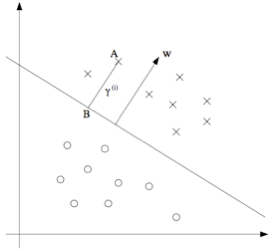
The figure shows the decision boundary corresponding to $(w, b)$. Its direction of tilt (that is, the normal direction) is the direction of the vector $w$. The vector $w$ is orthogonal to the separating hyperplane (the angle between them is $90^\circ$). (You should convince yourself that this must be the case.) Suppose $A$ is the point shown in the figure, representing a training example whose input features are $x^{(i)}$ and whose label is $y^{(i)} = 1$. The distance $\gamma^{(i)}$ from this point to the decision boundary is the length of the segment $AB$.
How do we find the value of $\gamma^{(i)}$? The vector $w/\parallel w\parallel$ is a unit-length vector pointing in the same direction as $w$. Since the point $A$ represents $x^{(i)}$, we can find a point $B$ located at $x^{(i)} - \gamma^{(i)} \times w/\parallel w\parallel$. This point $B$ lies exactly on the decision boundary, and every $x$ on that line satisfies $w^T x + b = 0$, so
$$ w^T(x^{(i)}-\gamma^{(i)}\frac{w}{\parallel w\parallel })+b=0 $$Solving the equation above for $\gamma^{(i)}$ gives
$$ \gamma^{(i)}=\frac{w^Tx^{(i)}+b}{\parallel w\parallel }=(\frac{w}{\parallel w\parallel })^Tx^{(i)}+\frac{b}{\parallel w\parallel } $$This solution is for the case, shown in the figure, in which $A$ is a positive training example, so lying on the “positive” side is the desirable situation. More generally, we define the geometric margin of $(w, b)$ with respect to the training example $(x^{(i)}, y^{(i)})$ by
$$ \gamma^{(i)}=y^{(i)}((\frac{w}{\parallel w\parallel })^Tx^{(i)}+\frac{b}{\parallel w\parallel }) $$Note that if $\parallel w\parallel = 1$, then the functional margin equals the geometric margin — this is one way to relate the two notions of margin. Furthermore, the geometric margin is unaffected by scaling the parameters. That is, if we replace $w$ by $2w$ and $b$ by $2b$, the geometric margin does not change. This property will be useful shortly. In particular, because of this invariance to parameter scaling, when we try to fit $w$ and $b$ to a data set we may impose an arbitrarily chosen scaling constraint on $w$ without changing anything important. For example, we may set $\parallel w\parallel = 1$, or $|w_1| = 5$, or $|w_1 + b| + |w_2| = 2$, and so on. Any of these can be satisfied just by scaling $w$ and $b$.
Finally, given a training set $S = \{(x^{(i)}, y^{(i)}); i = 1, ..., m\}$, we likewise define the geometric margin of $(w, b)$ with respect to $S$ to be the smallest geometric margin of the individual training examples:
$$ \gamma=\min_{i=1,...,m}\gamma^{(i)} $$4 The optimal margin classifier
Given a training set, the discussion above makes it natural to try, as a first priority, to find a decision boundary that maximizes the (geometric) margin. That reflects a series of high-confidence classification predictions on the training set, and a good “fit” to the training data. The classifier obtained in this way separates the positive and negative training examples, with a “gap” between them — namely the geometric margin.
So far we have assumed that the given training set is linearly separable. That is, the positive and negative examples can be divided by some separating hyperplane. How do we find the choice that yields the largest geometric margin? We can pose the following optimization problem:
$$ \begin{aligned} max_{\gamma,w,b} \quad& \gamma \\ s.t. \quad &y^{(i)}(w^Tx^{(i)}+b) \geq \gamma,\quad i=1,...,m\\ &\parallel w\parallel =1 \\ \end{aligned} $$That is, we maximize $\gamma$ so that every training example has functional margin at least $\gamma$. The constraint $\parallel w\parallel = 1$ also guarantees that the functional margin equals the geometric margin, so we are further guaranteed that every geometric margin is at least $\gamma$. Solving the optimization problem above therefore yields the $(w, b)$ of largest possible geometric margin for the training set.
If we could solve the optimization problem above, we would be done. But the constraint “$\parallel w\parallel = 1$” is awkward: it is non-convex, and the problem is clearly not one we can simply hand to some piece of standard optimization software. So we reformulate the problem to make it easier to solve. For example:
$$ \begin{aligned} max_{\hat\gamma,w,b} \quad& \frac{\hat \gamma}{\parallel w\parallel } \\ s.t. \quad &y^{(i)}(w^Tx^{(i)}+b) \geq \gamma,\quad i=1,...,m\\ \end{aligned} $$Here we maximize $\hat\gamma / \parallel w\parallel$ so that every functional margin is at least $\hat\gamma$. Because the geometric margin and the functional margin are related by $\gamma = \hat\gamma / \parallel w\parallel$, this gives the result we want. It also removes the awkward constraint $\parallel w\parallel = 1$. Unfortunately, we now have an awkward (and still non-convex) objective $\hat\gamma / \parallel w\parallel$, and there is still no off-the-shelf software that can solve an optimization problem of this form.
Let us continue. Recall that we may impose an arbitrary scaling constraint on $w$ and $b$ without changing anything essential. We now use that important property. We introduce a scaling constraint so that the functional margin of $w, b$ with respect to the training set equals $1$:
$$ \hat \gamma =1 $$Multiplying $w$ and $b$ by some constant multiplies the functional margin by the same constant. This really is a scaling constraint, and it can be met just by scaling $w$ and $b$. Applying this property to the optimization problem above, and noting that $\parallel w\parallel^2$ is minimized precisely when $\hat\gamma / \parallel w\parallel = 1 / \parallel w\parallel$ is maximized, we obtain the following optimization problem:
$$ \begin{aligned} min_{\gamma,w,b} \quad& \frac{1}{2}\parallel w\parallel ^2 \\ s.t. \quad &y^{(i)}(w^Tx^{(i)}+b) \geq 1,\quad i=1,...,m\\ \end{aligned} $$After this transformation, the problem is easy to solve. It has a convex quadratic objective and only linear constraints. Solving it gives the optimal margin classifier. The optimization problem can be solved with commercial quadratic programming (QP) code.$^1$
1 You may be more familiar with linear programming, which applies to optimization problems with linear objectives and linear constraints. QP software applies quite broadly, including to the case of a convex quadratic objective and linear constraints.
We could almost say that the problem has been solved. Next we digress and discuss Lagrange duality. That leads to the dual form of our optimization problem. The dual form will play an important role when we later use kernels, which can efficiently build an optimal margin classifier for data in extremely high-dimensional spaces. From the dual form we can also derive a very efficient algorithm for the optimization problem above, and that algorithm is usually better than generic QP software.
5 Lagrange duality
Let us set SVMs and the maximum-margin classifier aside for a moment, and talk about how to solve constrained optimization problems.
Consider a problem of the following form:
$$ \begin{aligned} min_w \quad & f(w)& \\ s.t. \quad &h_i(w) =0,\quad i=1,...,l\\ \end{aligned} $$Some readers may remember that this problem can be solved by the method of Lagrange multipliers. (It is fine if you have not seen it.) In that method we define the Lagrangian to be
$$ L(w,\beta)=f(w)+\sum^l_{i=1}\beta_i h_i(w) $$In the equation above, the $\beta_i$ are called Lagrange multipliers. We then take partial derivatives of $L$ and set them to zero:
$$ \frac{\partial L }{\partial w_i} =0; \quad \frac{\partial L }{\partial \beta_i} =0; $$and solve for the corresponding $w$ and $\beta$. In this section we generalize the method to constrained optimization problems that contain both inequality constraints and equality constraints. Because of limited space, we cannot do the theory of Lagrange duality justice in this course.$^2$ We will still give the main ideas and a few conclusions, which will be used for the optimal margin classifier’s optimization problem later.
2 Readers interested in Lagrange duality who want to know more may consult R. T. Rockefeller (1970), Convex Analysis, Princeton University Press.
The following is what we call the primal optimization problem:
$$ \begin{aligned} min_w \quad & f(w)& \\ s.t. \quad & g_i(w) \le 0,\quad i=1,...,k\\ & h_i(w) =0,\quad i=1,...,l\\ \end{aligned} $$To solve a problem of this form, we first define the generalized Lagrangian:
$$ L(w,\alpha,\beta)=f(w)+\sum^k_{i=1}\alpha_ig_i(w)+\sum^l_{i=1}\beta_ih_i(w) $$In the expression above, both $\alpha_i$ and $\beta_i$ are Lagrange multipliers. Consider the following quantity:
$$ \theta_{P}(w)=\max_{\alpha,\beta:\alpha_i \geq 0}L(w,\alpha,\beta) $$The “$P$” above is short for “primal”. Suppose some $w$ has already been given. If $w$ fails to satisfy some primal constraint (for example, $g_i(w) > 0$ or $h_i(w) \neq 0$ for some $i$), then we can show that
$$ \begin{aligned} \theta_P(w)&=\max_{\alpha,\beta:\alpha_i \geq 0} f(w)+\sum^k_{i=1}\alpha_ig_i(w)+\sum^l_{i=1}\beta_ih_i(w) &\text{(1)}\\ &= \infty &\text{(2)}\\ \end{aligned} $$Conversely, if a particular value of $w$ does satisfy the constraints, then $\theta_P(w) = f(w)$. In summary:
$$ \theta_P(w)= \begin{cases} f(w) & \text {if w satisfies primal constraints} \\ \infty & \text{otherwise} \end{cases} $$Thus, if a value of $w$ satisfies the primal constraints, the value of $\theta_P$ equals the objective of this optimization problem, whereas if the constraints cannot be satisfied, the value of $\theta_P$ is positive infinity. This leads further to the following minimization problem:
$$ \min_w \theta_P(w)=\min_w \max_{\alpha,\beta:\alpha_i\geq0} L(w,\alpha,\beta) $$This newly posed problem has the same solution as the earlier primal constrained problem, so it is the same problem. For use later on, we define here the optimal value of the objective, $p^\ast = \min_w \theta_P(w)$. We call this the value of the primal problem.
Next we look at a slightly different problem. We define $\theta_D$ as follows:
$$ \theta_D(\alpha,\beta)=\min_w L(w,\alpha,\beta) $$In the expression above, “$D$” is short for “dual”. Note that in the definition of $\theta_P$ we optimized over $\alpha$ and $\beta$ (taking a maximum), whereas here we take the minimum over $w$.
We can now state the dual optimization problem:
$$ \max_{\alpha,\beta:\alpha_i\geq 0} \theta_D(\alpha,\beta) = \max_{\alpha,\beta:\alpha_i\geq 0} \min_w L(w,\alpha,\beta) $$This form is essentially the same as the primal problem we saw earlier. The only difference is that “max” and “min” have swapped places. We can also define the optimal value of the objective of this dual problem, namely $d^\ast = \max_{\alpha,\beta:\alpha_i\geq 0} \theta_D(w)$.
How are the primal constrained problem and the dual problem related? The following relation makes the connection easy to see:
$$ d^\ast = \max_{\alpha,\beta:\alpha_i\geq 0}\min_w L(w,\alpha,\beta) \leq \min_w \max_{\alpha,\beta:\alpha_i\geq 0}L(w,\alpha,\beta) =p^\ast $$(You should prove for yourself that, here and in what follows, the maximum of the minimum of a function — “max min” — is always less than or equal to the minimum of the maximum — “min max”.) Under certain particular conditions, however, the two are equal:
$$ d^\ast =p^\ast $$We can then solve the dual problem in place of the original primal problem. Let us now see what the particular conditions are that make the two equal.
Suppose that $f$ and the $g_i$ are convex,$^3$ and that the $h_i$ are affine.$^4$ Suppose further that $g$ is strictly feasible. This means that there exists some $w$ such that $g_i(w) < 0$ for every $i$.
3 When $f$ has a Hessian matrix, $f$ is convex if and only if that Hessian matrix is positive semidefinite. For example, $f(w) = w^T w$ is convex. Similarly, every linear function, and every affine function, is convex. (A non-differentiable function $f$ can also be convex, but we do not yet need such a general extended definition of convexity here.)
4 For example, there exist $a_i$ and $b_i$ such that $h_i(w) = a^T_i w + b_i$. “Affine” means roughly the same thing as “linear,” except that an extra intercept term $b_i$ is added on top of the linear transformation by the matrix.
Under the assumptions above, there must exist $w^\ast$, $\alpha^\ast$, and $\beta^\ast$ such that $w^\ast$ is a solution of the primal problem, $\alpha^\ast$ and $\beta^\ast$ are a solution of the dual problem, and $p^\ast = d^\ast = L(w^\ast, \alpha^\ast, \beta^\ast)$. Furthermore, these three, $w^\ast$, $\alpha^\ast$, and $\beta^\ast$, satisfy the Karush–Kuhn–Tucker conditions (KKT conditions), as follows:
$$ \begin{aligned} \frac{\partial}{\partial w_i}L(w^\ast,\alpha^\ast,\beta^\ast) &= 0,\quad i=1,...,n & \text{(3)}\\ \frac{\partial}{\partial \beta_i}L(w^\ast,\alpha^\ast,\beta^\ast)&= 0 ,\quad i=1,...,l & \text{(4)}\\ \alpha_i^\ast g_i(w^\ast)&= 0,\quad i=1,...,k & \text{(5)}\\ g_i(w^\ast)&\leq 0,\quad i=1,...,k & \text{(6)}\\ \alpha_i^\ast &\geq 0,\quad i=1,...,k &\text{(7)}\\ \end{aligned} $$Conversely, if some triple $w^\ast, \alpha^\ast, \beta^\ast$ satisfies the KKT conditions, then that triple is also a solution of the primal problem and of the dual problem.
Pay attention here to equation $(5)$, also called the KKT dual complementarity condition. This equation implies that when $\alpha_i^\ast > 0$, we have $g_i(w^\ast) = 0$. (That is, if the constraint $g_i(w) \leq 0$ is present, it should hold as an equality rather than as an inequality.) This equation is important in what follows, especially for showing that an SVM has only a small number of support vectors. When we study the SMO algorithm, the KKT dual complementarity condition can also be used as a convergence test.
6 Optimal margin classifiers
Earlier we arrived at the following (primal) optimization problem, used to find the optimal margin classifier:
$$ \begin{aligned} min_{\gamma,w,b} \quad & \frac12 \parallel w\parallel ^2\\ &\\ s.t. \quad &y^{(i)}(w^Tx^{(i)}+b)\geq 1,\quad i=1,...,m\\ \end{aligned} $$The constraints can be written in the following form:
$$ g_i(w)=-y^{(i)}(w^Tx^{(i)}+b)+1\leq 0 $$There is one such constraint for every example in the training set. Note that, by the KKT dual complementarity condition, we have $\alpha_i \geq 0$ only when the functional margin of a training example is exactly $1$ (the constraints corresponding to these examples all hold as equalities, that is, the corresponding $g_i(w) = 0$). As shown in the figure below, the solid line is the maximum-margin separating hyperplane.
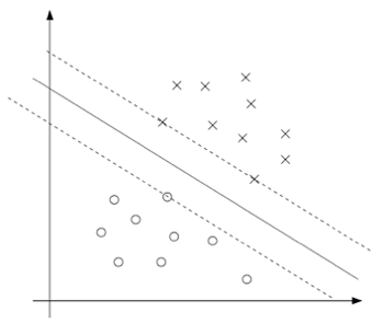
The examples with the smallest margins are exactly the points closest to the decision boundary. As the figure shows, there are three such points (one negative example, drawn as an open circle, and two positive examples, drawn as crosses). They lie on the dashed lines parallel to the decision boundary (the solid line). Therefore, in an optimal solution of this optimization problem, only the $\alpha_i$ corresponding to these three examples are nonzero. These three points are called the support vectors of this problem. The point of this phenomenon is that the number of support vectors can be smaller than the size of the training set, which will be used later.
Let us continue. We have already given the dual form of the problem. A key idea is that we next need to write the algorithm so that it involves only inner products $\langle x^{(i)}, x^{(j)}\rangle$ (which may also be read as $(x^{(i)})^T x^{(j)}$), that is, inner products of points in the input feature space. When we use the kernel trick, it is essential to express the algorithm in terms of inner products.
When we build the Lagrangian of the optimization problem, we have
$$ L(w,b,\alpha )=\frac{1}{2}\parallel w\parallel ^2 - \sum^m_{i=1}\alpha_i [y^{(i)}(w^Tx^{(i)}+b)-1] \qquad\text{(8)} $$Note that the Lagrange multipliers here include only the “$\alpha_i$” and not the “$\beta_i$”, because at this stage the problem has only inequality constraints.
Next we find the dual form of the problem. First we minimize $L(w, b, \alpha)$ by adjusting $w$ and $b$ while holding $\alpha$ fixed. That yields $\theta_D$. Concretely, we set the derivatives of $L$ with respect to $w$ and $b$ to zero. We then obtain
$$ \nabla_W L(w,b,\alpha)=w-\sum^m_{i=1}\alpha_i y^{(i)}x^{(i)} =0 $$Rewriting gives
$$ \begin{aligned} w=\sum^m_{i=1}\alpha_i y^{(i)}x^{(i)}\qquad\text{(9)} \end{aligned} $$Setting the derivative with respect to $b$ to zero gives
$$ \begin{aligned} \frac{\partial}{\partial b}L(w,b,\alpha)=\sum^m_{i=1}\alpha_i y^{(i)}=0 & \qquad \text{(10)} \end{aligned} $$Take the expression for $w$ given by equation $(9)$ above, substitute it into the Lagrangian, that is, into equation $(8)$, and simplify. This gives
$$L(w,b,\alpha)=\sum^m_{i=1}\alpha_i-\frac12 \sum^m_{i,j=1} y^{(i)}y^{(j)}\alpha_i\alpha_j(x^{(i)})^Tx^{(j)}-b\sum^m_{i=1}\alpha_i y^{(i)}$$From equation $(10)$ above, the last term must be $0$, so we can simplify further and obtain
$$L(w,b,\alpha)=\sum^m_{i=1}\alpha_i-\frac12 \sum^m_{i,j=1} y^{(i)}y^{(j)}\alpha_i\alpha_j(x^{(i)})^Tx^{(j)}$$Recall the equations we obtained earlier by minimizing $L$ with respect to $w$ and $b$. Combining those with the constraints $\alpha_i \geq 0$ (which hold throughout) and with equation $(10)$, we obtain the following dual optimization problem:
$$ \begin{aligned} max_\alpha \quad & W(\alpha) =\sum^m_{i=1}\alpha_i-\frac12\sum^m_{i,j=1}y^{(i)}y^{(j)}\alpha_i\alpha_j\langle x^{(i)} x^{(j)} \rangle\\ s.t. \quad & \alpha_i \geq 0,\quad i=1,...,m\\ & \sum^m_{i=1} \alpha_iy^{(i)}=0 \end{aligned} $$You should be able to verify that the conditions of this optimization problem are satisfied so that $p^\ast = d^\ast$ and the KKT conditions (equations $(3)$–$(7)$) hold. We can therefore solve the original primal problem by solving this dual problem. Concretely, we have built a maximization problem with the $\alpha_i$ as parameters. If we can solve that problem (that is, find an $\alpha$ that maximizes $W(\alpha)$ and satisfies the constraints), we can use equation $(9)$ to go back to the original problem and find the optimal $w$ as a function of $\alpha$. Once we have $w^\ast$, we return to the primal problem and can find the optimal value of the intercept term $b$ directly:
$$ \begin{aligned} b^\ast =- \frac{ \max_{i:y^{(i)}=-1}w^{\ast T}x^{(i)}+\min_{i:y^{(i)}=-1}w^{\ast T}x^{(i)} }{2} & \text{ (11)}\\ \end{aligned} $$(Prove this yourself.) Before going on, look again at equation $(9)$, which expresses the optimal value of $w$ in terms of $\alpha$ (at its optimal value). Suppose we have already fit the model parameters on a training set, and we now want to predict the target value of a new input $x$. We compute $w^T x + b$, and if the value we obtain is greater than $0$, we predict $y = 1$. Using equation $(9)$, this same property can also be written
$$ \begin{aligned} w^Tx+b&= (\sum^m_{i=1}\alpha_i y^{(i)}x^{(i)})^Tx+b & \text{(12)}\\ &= \sum^m_{i=1}\alpha_i y^{(i)}\langle x^{(i)},x \rangle+b & \text{(13)}\\ \end{aligned} $$In that case, to make a prediction, once the $\alpha_i$ have been found, we must compute a quantity that depends only on the inner products of the new input features $x$ with each point in the training set. We have also already seen that $\alpha_i$ is $0$ except for the support vectors. Many terms in the sum above are therefore $0$. We then need only the inner products of $x$ with the support vectors — so the computation actually uses only a small portion of the data, rather than the entire training set — and we can evaluate equation $(13)$. The result can then be used for prediction.
By examining the dual form of the optimization problem, we have gained a deeper understanding of the structure of the problem we need to solve, and we have also written the entire algorithm in terms of inner products between input feature vectors. In the next section we make full use of this, and then apply kernels to our classification problem. The resulting algorithm, the support vector machine algorithm, will be able to learn efficiently in very high-dimensional spaces.
7 Kernels
When we discussed linear regression earlier, we met a problem in which the input $x$ was the living area of a house, and we considered using the features $x$, $x^2$, and $x^3$ to fit a cubic function. To distinguish the two collections of quantities, we call the “raw” input values the input attributes of a problem, for example the living area $x$. When these values are mapped to some other collection of quantities and passed to the learning algorithm, the new values are called input features. (Unfortunately, different authors often use different names for the two, but in these notes we will try to keep the terminology consistent.) We also use $\phi$ to denote the feature mapping, that is, the mapping from the input attributes to the input features that are passed to the learning algorithm. In the living-area example just given, the feature mapping can be written
$$ \phi(x)=\left[ \begin{aligned}& x\\ & x^2\\ & x^3 \end{aligned}\right] $$Instead of simply applying an SVM directly to the raw input attributes $x$, we may try to use the new features $\phi(x)$ produced by the mapping. We only need to look back briefly at the earlier algorithm and replace every $x$ by $\phi(x)$.
Because the algorithm above can be written entirely in the form of inner products $\langle x, z\rangle$, this means we only need to replace every inner product above by the inner product $\langle\phi(x), \phi(z)\rangle$. More concisely, given a feature mapping $\phi$, we may define a corresponding kernel as follows:
$$ K(x,z)=\phi(x)^T\phi(z) $$Then we only need to replace every $\langle x, z\rangle$ used in the algorithm above by $K(x, z)$. That is enough: our algorithm then begins to learn using the feature mapping $\phi$.
Now, given a feature mapping $\phi$, it is easy to find $\phi(x)$ and $\phi(z)$, take their inner product, and thereby compute $K(x, z)$. But there is more. What is more interesting is that, in the usual case, computing this $K(x, z)$ is often very inexpensive, even when $\phi(x)$ itself is hard to compute (perhaps because the vector is extremely high-dimensional). In that setting, given a feature mapping $\phi$, we can use an SVM to learn in a high-dimensional feature space, and we may never have to go to the trouble of explicitly solving for the corresponding vector $\phi(x)$.
Let us look at an example. Suppose $x, z \in R^n$, and set
$$ K(x,z)= (x^Tz)^2 $$This can also be written as
$$ \begin{aligned} K(x,z)&=(\sum^n_{i=1}x_iz_i)(\sum^n_{j=1}x_jz_j)\\ &=\sum^n_{i=1}\sum^n_{j=1}x_ix_jz_iz_j\\ &=\sum^n_{i,j=1}(x_ix_j)(z_iz_j)\\ \end{aligned} $$Thus we see that $K(x, z) = \phi(x)^T \phi(z)$, where the feature mapping $\phi$ is given as follows (in this example $n = 3$):
$$ \phi(x)= \left[ \begin{aligned} &x_1x_1\\&x_1x_2\\&x_1x_3\\&x_2x_1\\&x_2x_2\\&x_2x_3\\ &x_3x_1\\&x_3x_2\\&x_3x_3 \end{aligned} \right] $$At this point we find that computing the high-dimensional $\phi(x)$ takes on the order of $O(n^2)$ computation, whereas computing $K(x, z)$ takes only on the order of $O(n)$ time, that is, time linear in the dimension of the input attributes.
A related kernel may be taken to be
$$ \begin{aligned} K(x,z)&= (x^Tz+c)^2 \\ &= \sum^n_{i,j=1}(x_ix_j)(z_iz_j)+\sum^n_{i=1}(\sqrt{2c}x_i)(\sqrt{2c}z_i)+c^2\\ \end{aligned} $$(Check this yourself.) The corresponding feature mapping is (again taking $n = 3$ as the example):
$$ \phi(x)= \left[ \begin{aligned} &x_1x_1\\&x_1x_2\\&x_1x_3\\&x_2x_1\\&x_2x_2\\&x_2x_3\\ &x_3x_1\\&x_3x_2\\&x_3x_3\\& \sqrt{2c}x_1\\& \sqrt{2c}x_2\\& \sqrt{2c}x_3\\&c\end{aligned} \right] $$Here the parameter $c$ controls the relative weighting of the first group, the $x_i$, and the second group, the $x_i x_j$.
Extending this one step further, the kernel $K(x, z) = (x^T z + c)^d$ corresponds to a feature mapping into a feature space of dimension $\left( \begin{aligned} n&+d \\ &d \end{aligned} \right)$, namely all monomials of the form $x_{i1}, x_{i2}, \ldots, x_{ik}$ of degree up to $d$. Yet even for a high-dimensional space of this kind, of dimension $O(n^d)$, computing $K(x, z)$ still takes only on the order of $O(n)$ time. We therefore do not need an explicit representation of the feature vectors in this very high-dimensional feature space.
Now let us look at the kernel from another point of view. Intuitively (and the intuition may be somewhat wrong, but that is all right; we can set that aside for now), if $\phi(x)$ and $\phi(z)$ are very close together, then we may expect $K(x, z) = \phi(x)^T \phi(z)$ to be large. Conversely, if $\phi(x)$ and $\phi(z)$ are far apart, for example nearly orthogonal, then $K(x, z) = \phi(x)^T \phi(z)$ may be small. We can therefore understand the kernel $K(x, z)$ as a measure of how close $\phi(x)$ and $\phi(z)$ are, or equivalently as a measure of how close $x$ and $z$ are.
With that intuition in hand, suppose you are trying some learning algorithm and have already constructed some function $K(x, z)$, and you are thinking that you might use this function to measure how close $x$ and $z$ are. For example, suppose you choose the following function:
$$ K(x,z)=\exp (- \frac{\parallel x-z\parallel ^2}{2\sigma^2 }) $$This function is a good measure of how close $x$ and $z$ are. When the two are close, the function value is near $1$; when they are far apart, the function value is near $0$. Can we use a function $K$ defined in this way as a kernel inside an SVM? In this particular example, the answer is yes. (This kernel is also called the Gaussian kernel, and it corresponds to an infinite-dimensional feature mapping $\phi$.) Generalizing one step further: given some function $K$, how can we determine whether this function is a valid kernel? For example, can we say that there exists some feature mapping $\phi$ such that $K(x, z) = \phi(x)^T \phi(z)$ for all $x$ and $z$?
For the moment, assume that $K$ is a valid kernel, corresponding to some feature mapping $\phi$. Then consider some finite set of $m$ points $\{x^{(1)}, \ldots, x^{(m)}\}$ (this set does not have to be a training set), and let $K$ be a square $m \times m$ matrix defined by setting its $(i, j)$-th entry to $K_{ij} = K(x^{(i)}, x^{(j)})$. This matrix is called the kernel matrix. Notice that the symbol $K$ has been reused: it denotes both the kernel function $K(x, z)$ and the kernel matrix $K$, because the two are very closely related.
If $K$ is a valid kernel, then $K_{ij} = K(x^{(i)}, x^{(j)}) = \phi(x^{(i)})^T \phi(x^{(j)}) = \phi(x^{(j)})^T \phi(x^{(i)}) = K(x^{(j)}, x^{(i)}) = K_{ji}$, which shows that $K$ is a symmetric matrix. Furthermore, let $\phi_k(x)$ denote the $k$-th coordinate of the vector $\phi(x)$. Then for an arbitrary vector $z$ we have
$$ \begin{aligned} z^TKz&= \sum_i\sum_j z_iK_{ij}z_j \\ &= \sum_i\sum_j z_i\phi(x^{(i)})\phi(x^{(j)})z_j\\ &= \sum_i\sum_jz_i\sum_k \phi_k(x^{(i)})\phi_k(x^{(j)})z_j\\ &= \sum_k\sum_i\sum_j z_i\phi_k(x^{(i)})\phi_k(x^{(j)})z_j\\ &= \sum_k(\sum_i z_i\phi_k(x^{(i)}))^2\\ &\geq 0 \\ \end{aligned} $$From the second step through the last step, the derivation above uses the same trick as Question 1 of Problem Set 1. Since $z$ is arbitrary, this shows that the matrix $K$ is positive semidefinite ($K \geq 0$).
We have thus proved that if $K$ is a valid kernel (for example, if we assume that the function corresponds to some feature mapping $\phi$), then the corresponding kernel matrix $K \in R^{m \times m}$ is a symmetric positive semidefinite matrix. Going further, this is not merely a necessary condition for $K$ to be a valid kernel; it is also a sufficient condition. Such a kernel is called a Mercer kernel. The results shown below are due to Mercer.$^5$
5 Many textbooks state Mercer’s theorem in a more complicated way, involving $L2$ functions, but if the input attributes take values only in the real domain $R^n$, then the statement given here is equivalent.
Mercer’s theorem: Let a map $K: R^n \times R^n \rightarrow R$ be given. Then a necessary and sufficient condition for $K$ to be a valid Mercer kernel is that, for every $\{x^{(1)}, \ldots, x^{(m)}\}$ with $(m < \infty)$, the corresponding kernel matrix is symmetric positive semidefinite.
For a given function $K$, besides the earlier approach of finding a corresponding feature mapping $\phi$, the theorem above gives another way to verify whether the function is a valid kernel. Problem Set 2 contains many exercises; you can try them.
In the course we also briefly presented several examples of kernels. For example, in handwritten digit recognition, one is given an image of a handwritten digit ($0$–$9$), with $16 \times 16$ pixels, and the goal is to recognize which digit was written. Using either a simple polynomial kernel $K(x, z) = (x^T z)^d$ or the Gaussian kernel, the SVM showed excellent performance on this example. The result is rather surprising, because the input attribute $x$ is a $256$-dimensional vector, namely the vector of pixel intensities of the image to be recognized, and the system had no prior knowledge about visual judgment, not even about whether pixels are adjacent to one another. In another example from class, the object $x$ being classified is a string. For example, $x$ may be a sequence of amino acids joined together to form a protein. Building a reasonable and sufficiently “small” feature set that works for most machine learning algorithms is difficult, and the strings also have different lengths, which makes the difficulty greater still. There is a solution, however. Let $\phi(x)$ be a feature vector that counts the number of occurrences of each length-$k$ substring in $x$. If we consider strings made from the English alphabet, then there are $26^k$ such strings. In that case $\phi(x)$ is a $26^k$-dimensional vector; even when $k$ is not very large, this number becomes enormous and hard to compute effectively. (For example, $26^4 \approx 460000$.) Using a (dynamic-programming-style) string-matching algorithm, however, we can efficiently compute $K(x, z) = \phi(x)^T \phi(z)$. That is, we can handle a $26^k$-dimensional feature space implicitly, without ever having to compute the feature vectors in that space explicitly.
We have already been clear enough about the use of kernels in support vector machines, so we will not belabor the point here. One idea is still worth remembering: the use of kernels is by no means limited to the SVM algorithm. Specifically, whenever your learning algorithm can be written in a form that uses only inner products of the input attribute vectors, you can introduce a kernel $K$, replacing those inner products by $K(x, z)$, and thereby “power up” your algorithm so that it runs efficiently in the high-dimensional feature space corresponding to $K$. Combining a kernel with the perceptron also produces the kernel perceptron algorithm. Many of the algorithms we will study later can be treated in the same way. This method is the kernel trick.
8 Regularization and the non-separable case
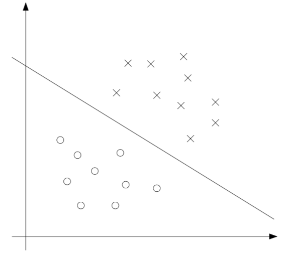
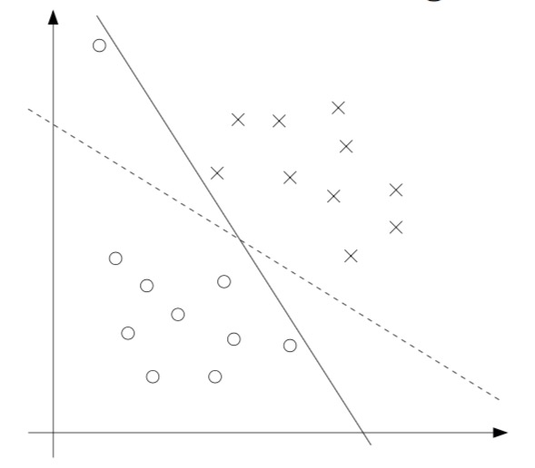
So far, our derivation of the SVM has rested on an assumption, namely that all of the data are linearly separable. Mapping the data into a high-dimensional feature space through a feature mapping $\phi$ usually increases the probability that the data are separable, but we still cannot guarantee that the data can always be separated. Moreover, in some cases, finding a separating hyperplane is not necessarily what we are after, because outliers can appear quite easily. For example, the figure below shows an optimal margin classifier. If a single outlier lands in the upper-right region (as shown in the right-hand figure), the decision boundary shifts markedly, and the margin of the classifier also shrinks by a great deal.
To make the algorithm apply to data sets that are not linearly separable, and to make it somewhat less sensitive to outliers, we reformulate our optimization problem (using $l1$ regularization) as follows:
$$ \begin{aligned} min_{\gamma,w,b}& \frac 12 \parallel w\parallel ^2+C\sum^m_{}\xi_i \\ s.t.& y^{(i)}(w^Tx^{(i)}+b) \geq1-\xi_i,i=1,...,m\\ & \xi_i \geq 0 ,i=1,...,m \end{aligned} $$This allows the data set to contain cases in which the (functional) margin is less than $1$. If an example has functional margin $1 - \xi_i$ (where $\xi \geq 0$), we must then pay $C\xi_i$ as the cost of the objective function being increased. The quantity $C$ is a parameter that controls the relative weight. The control is a tradeoff between a pair of goals: one is to make $\parallel w\parallel^2$ as small as possible (as the examples in earlier sections showed, this maximizes the margin), and the other is to ensure that the great majority of examples have functional margin at least $1$.
As usual, we write down the Lagrangian:
$$ L(w,b,\xi,\alpha,r)=\frac12w^Tw+C\sum^m_{i=1}\xi_i-\sum^m_{i=1}\alpha_i[y^{(i)}(x^Tw+b)-1+\xi_i]-\sum^m_{i=1}r_i\xi_i $$In the expression above, both $\alpha_i$ and $r_i$ are Lagrange multipliers (constrained to be nonnegative, $\geq 0$). This time we will not derive the dual form in detail. As usual, however, we set the derivatives with respect to $w$ and $b$ to zero, substitute them back, and simplify, and thereby obtain the following dual form of the problem:
$$ \begin{aligned} \max_\alpha \quad & W(\alpha) =\sum^m_{i=1}\alpha_i-\frac12\sum^m_{i,j=1}y^{(i)}y^{(j)}\alpha_i\alpha_j \langle x^{(i)},x^{(j)} \rangle \\ s.t. \quad & 0\leq \alpha_i \leq C,i=1,...,m\\ & \sum^m_{i=1}\alpha_iy^{(i)}=0 \\ \end{aligned} $$As before, we can still express $w$ in terms of the $\alpha_i$, as in equation $(9)$. After solving the dual problem, we can then use equation $(13)$ to make our predictions. Note one remarkable point: after $l1$ regularization is added, the only change to the dual problem is that the original constraint $0 \leq \alpha_i$ now becomes $0 \leq \alpha_i \leq C$. The computation of $b^\ast$ is also affected and changes (equation (11) is no longer valid). For the details, see the next section, or read Platt’s paper.
In addition, the KKT dual complementarity conditions (which the next section uses to test convergence of the SMO algorithm) are
$$ \begin{aligned} \alpha_i&= 0 &\implies y^{(i)}(w^Tx^{(i)}+b)\ge 1 \qquad &\text{(14)}\\ \alpha_i&= C &\implies y^{(i)}(w^Tx^{(i)}+b)\le 1 \qquad &\text{(15)}\\ 0\leq \alpha_i& \leq C &\implies y^{(i)}(w^Tx^{(i)}+b) = 1 \qquad &\text{(16)}\\ \end{aligned} $$All that remains is to give an algorithm that actually solves this dual problem. We take up that problem in the next section.
9 The SMO optimization algorithm
SMO is short for sequential minimal optimization. The algorithm was proposed in 1998 by John Platt at Microsoft Research. For the dual problem derived from the SVM, it provides an efficient method of solution. We first discuss the coordinate ascent algorithm. That algorithm is interesting in its own right, and it is also a step used to derive the SMO algorithm.
9.1 Coordinate ascent
Suppose we want to solve the following unconstrained optimization problem:
$$ \max_\alpha W(\alpha_1,\alpha_2,...,\alpha_m) $$Here $W$ is some function of the parameters $\alpha_i$. For the moment we ignore any relationship between this problem and the support vector machine. Earlier we already learned two optimization algorithms, gradient descent and Newton’s method. The new optimization algorithm below is called coordinate ascent:
$$ \begin{aligned} &Repeat\ until\ convergence:\ \{ \\ &\qquad For\quad i=1,...,m, \{ \\ &\qquad\qquad\alpha_i:= \arg \max_{\hat \alpha_i}W(\alpha_1,...,\alpha_{i-1},\hat\alpha_i,\alpha_{i+1},...,\alpha_m) \\ &\qquad\} \\ &\} \end{aligned} $$As the display above shows, in the innermost loop the algorithm holds fixed every variable except some particular $\alpha_i$, and then re-optimizes $W$ by adjusting the parameter $\alpha_i$. In the version of the algorithm given here, the innermost loop re-optimizes the variables in the order $\alpha_1, \alpha_2, \ldots, \alpha_m, \alpha_1, \alpha_2, \ldots$. A more sophisticated version might choose some other order. For example, we may choose the next variable to update according to which one we expect to allow us to make the largest increase in $W(\alpha)$.
If, inside the function $W$, the “$\arg\max$” in the innermost loop can be carried out very efficiently, then coordinate ascent becomes quite an efficient algorithm. Below is a sketch of coordinate ascent:
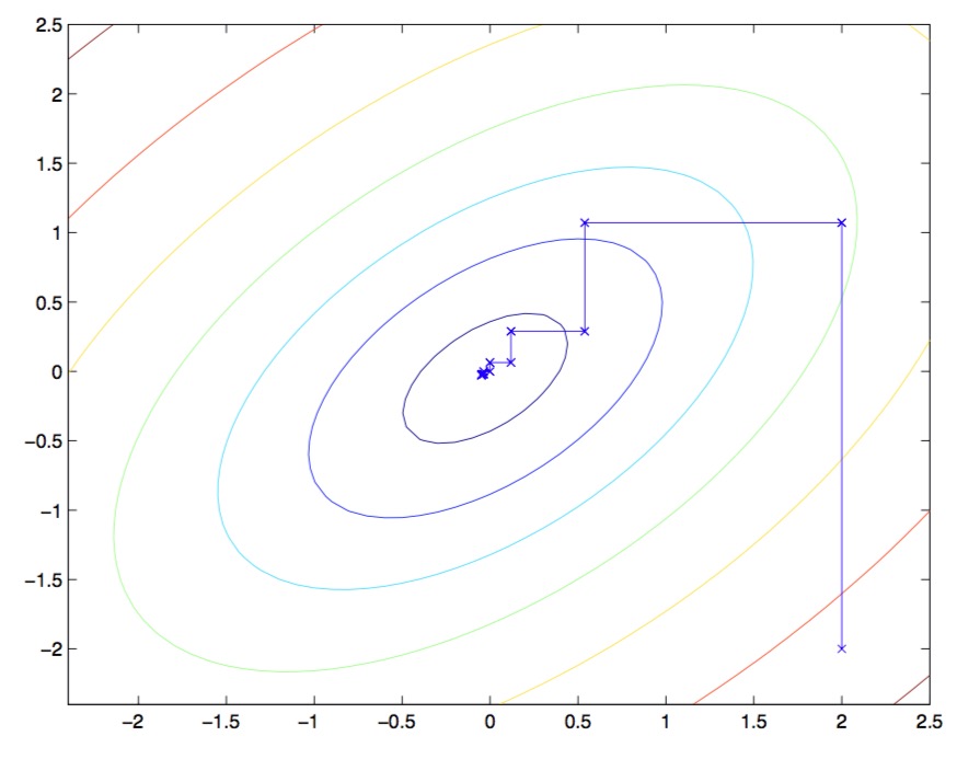
The ellipses in the figure are the contours of the quadratic function we want to optimize. Coordinate ascent is initialized at $(2, -2)$, and the figure also marks the path to the global maximum. Note that at every step of coordinate ascent the direction of movement is parallel to one of the coordinate axes, because only one variable is optimized at a time.
9.2 The SMO optimization algorithm
Next we briefly derive the SMO algorithm, as a close to the discussion of the SVM. Some of the concrete details are omitted and left to the homework; other material can be found in the printed handout distributed in class.
The following is a (dual) optimization problem:
$$ \begin{aligned} \max_\alpha \quad & W(\alpha)= \sum^m_{i=1}\alpha_i-\frac12 \sum^m_{i,j=1}y^{(i)}y^{(j)}\alpha_i\alpha_j\langle x^{(i)},x^{(j)}\rangle & \text{(17)}\\ s.t.\quad & 0\leq \alpha_i \leq C,i=1,...,m& \text{(18)}\\ & \sum^m_{i=1}\alpha_iy^{(i)}=0& \text{(19)}\\ \end{aligned} $$Suppose we have a set of $\alpha_i$ satisfying the constraints $(18)$–$(19)$. Next, suppose we hold the values of $\alpha_2, \ldots, \alpha_m$ fixed and take one step of coordinate ascent, re-optimizing the objective with respect to $\alpha_1$. Can we solve that? Unfortunately, no, because constraint $(19)$ means that
$$ \alpha_1y^{(1)}=-\sum^m_{i=2}\alpha_iy^{(i)} $$Alternatively, we may multiply both sides by $y^{(1)}$ and obtain the following equation, which is equivalent to the one above:
$$ \alpha_1=-y^{(1)}\sum^m_{i=2}\alpha_iy^{(i)} $$(This step uses the fact that $y^{(1)} \in \{-1, 1\}$, so $(y^{(1)})^2 = 1$.) Thus $\alpha_1$ is determined by the other $\alpha_i$. If we hold $\alpha_2, \ldots, \alpha_m$ fixed, there is no way to make any change to the value of $\alpha_1$, or else constraint $(19)$ of the optimization problem would fail.
Therefore, if we want to update some of the values among the $\alpha_i$, we must update at least two of them at the same time, so that the constraints remain satisfied. This situation gives rise to the SMO algorithm, which, stated briefly, is as follows:
Repeat until convergence {
Select some pair $\alpha_i$ and $\alpha_j$ to update on the next iteration (using a heuristic that tries to pick the two that will allow us to make the biggest progress toward the global maximum).
Re-optimize $W(\alpha)$ using the corresponding $\alpha_i$ and $\alpha_j$, while holding the other values $\alpha_k$ fixed ($k \neq i, j$).
}
We can test convergence of this algorithm by checking whether the KKT dual complementarity conditions are satisfied to within some convergence tolerance parameter tol. Here tol is the convergence tolerance parameter, and it is usually set to about $0.01$ to $0.001$. (For further details, see the references and the pseudocode.)
A key reason that the SMO algorithm is efficient is that the updates of $\alpha_i$ and $\alpha_j$ can be computed very efficiently. We now briefly outline the idea behind deriving that efficient update.
Suppose we currently have some $\alpha_i$ satisfying constraints $(18)$–$(19)$. If we decide to hold $\alpha_3, \ldots, \alpha_m$ fixed and then re-optimize $W(\alpha_1, \alpha_2, \ldots, \alpha_m)$ using this pair $\alpha_1$ and $\alpha_2$, the paired update is again in order to satisfy the constraints. From constraint $(19)$ we obtain
$$ \alpha_1y^{(1)} + \alpha_2y^{(2)} = -\sum^m_{i=3}\alpha_iy^{(i)} $$The right-hand side is fixed, because we have already fixed the values of $\alpha_3, \ldots, \alpha_m$, so we may abbreviate the right-hand side as a constant $\zeta$:
$$ \alpha_1y^{(1)} + \alpha_2y^{(2)} = \zeta \qquad \text{(20)} $$We can then use the following figure to depict the constraints on $\alpha_1$ and $\alpha_2$:
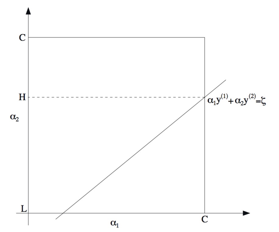
From constraint $(18)$, $\alpha_1$ and $\alpha_2$ must lie in the box $[0, C] \times [0, C]$ shown in the figure. The figure also contains the line $\alpha_1 y^{(1)} + \alpha_2 y^{(2)} = \zeta$, and we know that $\alpha_1$ and $\alpha_2$ must lie on this line. Note also that the constraints above further imply $L \leq \alpha_2 \leq H$; otherwise $(\alpha_1, \alpha_2)$ cannot satisfy, at the same time, both the constraint of lying inside the box and the constraint of lying on the line. In the example above, $L = 0$. But, considering the shape and direction of the line $\alpha_1 y^{(1)} + \alpha_2 y^{(2)} = \zeta$, this value $L = 0$ is not necessarily the best one. In general, however, the possible values of $\alpha_2$ for which $\alpha_1$ and $\alpha_2$ lie inside the box $[0, C] \times [0, C]$ have a lower bound $L$ and an upper bound $H$.
Using equation $(20)$, we can also write $\alpha_1$ as a function of $\alpha_2$:
$$ \alpha_1=(\zeta-\alpha_2y^{(2)})y^{(1)} $$(Check this derivation yourself. It again uses the fact that $y^{(1)} \in \{-1, 1\}$, so $(y^{(1)})^2 = 1$.) The objective $W(\alpha)$ can therefore be written
$$ W(\alpha_1,\alpha_2,...,\alpha_m)=W((\zeta-\alpha_2y^{(2)})y^{(1),\alpha_2,...,\alpha_m}) $$Treating $\alpha_3, \ldots, \alpha_m$ as constants, you can show that the function above is really just a quadratic function of $\alpha_2$. That is, it can in fact be written in the form $a\alpha_2^2 + b\alpha_2 + c$, with parameters $a$, $b$, and $c$. If we temporarily ignore the box constraint (18) (that is, $L \leq \alpha_2 \leq H$), then it is easy to find the maximum of this quadratic by setting the derivative to zero, and then to solve. Let $\alpha_2^{new, unclipped}$ denote the resulting value of $\alpha$. You should prove for yourself that if we want to maximize the function $W$ with respect to $\alpha_2$, subject to the box constraint, then we can take the value $\alpha_2^{new, unclipped}$ and “clip” it so that it lies in the interval $[L, H]$. Finding the optimal value in this way gives
$$ \alpha_2^{new}= \begin{cases} H & if \quad\alpha_2^{new, unclipped}> H\\ \alpha_2^{new, unclipped} & if \quad L\leq \alpha_2^{new, unclipped}\leq H\\ L & if \quad \alpha_2^{new, unclipped}There are a few other details as well. They are all fairly simple, but we will not cover them here; go and read Platt’s paper yourself. One is the heuristic choice of the $\alpha_i$ and $\alpha_j$ to be used for the next update. The other is how to update $b$ while the SMO algorithm is running.