
| |
Pandas Indexing
I. Indexers
1. Column Indexing in a Table
Column indexing is the most common form of indexing and is typically done with []. Using [column name] extracts the corresponding column from a DataFrame and returns a Series—for example, selecting the name column:
| |
0      Gaopeng Yang
1    Changqiang You
2           Mei Sun
3      Xiaojuan Sun
4       Gaojuan You
Name: Name, dtype: object
To fetch multiple columns, pass a [list of column names]; the result is a DataFrame. Here we extract the gender and name columns:
| |
| Gender | Name | |
|---|---|---|
| 0 | Female | Gaopeng Yang |
| 1 | Male | Changqiang You |
| 2 | Male | Mei Sun |
| 3 | Female | Xiaojuan Sun |
| 4 | Male | Gaojuan You |
In addition, when selecting a single column whose name contains no spaces, you can use .column_name, which is equivalent to [column name]:
| |
0      Gaopeng Yang
1    Changqiang You
2           Mei Sun
3      Xiaojuan Sun
4       Gaojuan You
Name: Name, dtype: object
2. Row Indexing of a Series
[a] Series with string indices
To retrieve the element corresponding to a single index label, use [item]. If only one value matches, that scalar is returned; when several values match, a Series comes back:
| |
a    1
a    3
a    4
a    5
dtype: int64
| |
2
To fetch the elements for several index labels at once, use [a list of items]:
| |
c    6
b    2
dtype: int64
When you want the elements between two index labels that each occur only once in the whole index, a slice does the job; note that such a slice includes both endpoints:
| |
c    6
a    4
b    2
dtype: int64
If the endpoint labels appear more than once, the index must be sorted before slicing:
| |
KeyError("Cannot get left slice bound for non-unique label: 'a'")
| |
a    1
a    3
a    4
a    5
b    2
dtype: int64
[b] Series with integer indices
When reading data without explicitly naming a column as the index, pandas creates a default integer index starting at 0. Of course, any set of integers of the right length can serve as an index.
As with strings, using [int] or [int_list] retrieves the element values associated with those index labels:
| |
1    a
1    c
dtype: object
| |
2    d
3    b
dtype: object
An integer slice, by contrast, selects values by position; like a Python slice, it excludes the right endpoint:
| |
3    b
2    d
dtype: object
[WARNING] A note on index types
To stay out of trouble, avoid using pure floats or any mixed type (a blend of strings, integers, floats, and so on) as an index. Doing so may raise errors or produce unexpected results during specific operations, and there is no real-world motive for it in data analysis either.
[END]
3. The loc indexer
We have looked at selecting columns of a DataFrame; next we turn to selecting rows. For a table there are two indexers: the loc indexer, based on element labels, and the iloc indexer, based on position.
The general form of the loc indexer is loc[*, *], where the first * selects rows and the second selects columns. If you omit the second position and write loc[*], that single * refers to row filtering. Each * slot accepts five kinds of legal objects: a single element, a list of elements, a slice of elements, a Boolean list, and a function; we explain them in turn below.
To demonstrate these operations, we first use set_index to make the Name column the index; other uses of this function are covered in the multi-index chapter.
| |
| School | Grade | Gender | Weight | Transfer | |
|---|---|---|---|---|---|
| Name | |||||
| Gaopeng Yang | Shanghai Jiao Tong University | Freshman | Female | 46.0 | N |
| Changqiang You | Peking University | Freshman | Male | 70.0 | N |
| Mei Sun | Shanghai Jiao Tong University | Senior | Male | 89.0 | N |
| Xiaojuan Sun | Fudan University | Sophomore | Female | 41.0 | N |
| Gaojuan You | Fudan University | Sophomore | Male | 74.0 | N |
[a] * is a single element
Here the corresponding row or column is taken directly. If the element is repeated in the index the result is a DataFrame; otherwise it is a Series:
| |
| School | Grade | Gender | Weight | Transfer | |
|---|---|---|---|---|---|
| Name | |||||
| Qiang Sun | Tsinghua University | Junior | Female | 53.0 | N |
| Qiang Sun | Tsinghua University | Sophomore | Female | 40.0 | N |
| Qiang Sun | Shanghai Jiao Tong University | Junior | Female | NaN | N |
| |
School      Shanghai Jiao Tong University
Grade                              Junior
Gender                             Female
Weight                               53.0
Transfer                                N
Name: Quan Zhao, dtype: object
You can also select rows and columns at the same time:
| |
Name
Qiang Sun              Tsinghua University
Qiang Sun              Tsinghua University
Qiang Sun    Shanghai Jiao Tong University
Name: School, dtype: object
| |
'Shanghai Jiao Tong University'
[b] * is a list of elements
Here we fetch all rows or columns corresponding to the element values in the list:
| |
| School | Gender | |
|---|---|---|
| Name | ||
| Qiang Sun | Tsinghua University | Female |
| Qiang Sun | Tsinghua University | Female |
| Qiang Sun | Shanghai Jiao Tong University | Female |
| Quan Zhao | Shanghai Jiao Tong University | Female |
[c] * is a slice
Earlier, when discussing Series with string indices, we saw that a slice is allowed when the start and end labels are unique; it includes both endpoints, and raises an error if they are not unique:
| |
| School | Grade | Gender | |
|---|---|---|---|
| Name | |||
| Gaojuan You | Fudan University | Sophomore | Male |
| Xiaoli Qian | Tsinghua University | Freshman | Female |
| Qiang Chu | Shanghai Jiao Tong University | Freshman | Female |
| Gaoqiang Qian | Tsinghua University | Junior | Female |
Note that when a DataFrame uses an integer index, integer slicing follows the same rules as string slicing above: it is an element slice that includes both endpoints, and neither endpoint may be a duplicated value.
| |
| School | Grade | Gender | Weight | Transfer | |
|---|---|---|---|---|---|
| 5 | Fudan University | Junior | Female | 46.0 | N |
| 4 | Tsinghua University | Senior | Female | 50.0 | N |
| 3 | Shanghai Jiao Tong University | Senior | Female | 45.0 | N |
| |
| School | Grade | Gender | Weight | Transfer |
|---|
[d] * is a Boolean list
In real data work, filtering rows by conditions is extremely common. The Boolean list passed to loc has the same length as the DataFrame; rows where the list is True are kept, while those marked False are dropped.
For example, to select students weighing more than 70 kg:
| |
| School | Grade | Gender | Weight | Transfer | |
|---|---|---|---|---|---|
| Name | |||||
| Mei Sun | Shanghai Jiao Tong University | Senior | Male | 89.0 | N |
| Gaojuan You | Fudan University | Sophomore | Male | 74.0 | N |
| Xiaopeng Zhou | Shanghai Jiao Tong University | Freshman | Male | 74.0 | N |
| Xiaofeng Sun | Tsinghua University | Senior | Male | 71.0 | N |
| Qiang Zheng | Shanghai Jiao Tong University | Senior | Male | 87.0 | N |
The element lists mentioned earlier can equally be expressed as a Boolean list returned by isin—for instance, selecting all freshmen and seniors:
| |
| School | Grade | Gender | Weight | Transfer | |
|---|---|---|---|---|---|
| Name | |||||
| Gaopeng Yang | Shanghai Jiao Tong University | Freshman | Female | 46.0 | N |
| Changqiang You | Peking University | Freshman | Male | 70.0 | N |
| Mei Sun | Shanghai Jiao Tong University | Senior | Male | 89.0 | N |
| Xiaoli Qian | Tsinghua University | Freshman | Female | 51.0 | N |
| Qiang Chu | Shanghai Jiao Tong University | Freshman | Female | 52.0 | N |
Compound conditions can be built by combining | (OR), & (AND), and ~ (NOT)—for example, seniors at Fudan University who weigh more than 70 kg, or non-senior male students at Peking University who weigh more than 80 kg:
| |
| School | Grade | Gender | Weight | Transfer | |
|---|---|---|---|---|---|
| Name | |||||
| Qiang Han | Peking University | Freshman | Male | 87.0 | N |
| Chengpeng Zhou | Fudan University | Senior | Male | 81.0 | N |
| Changpeng Zhao | Peking University | Freshman | Male | 83.0 | N |
| Chengpeng Qian | Fudan University | Senior | Male | 73.0 | Y |
[Practice]
select_dtypes is a handy function that picks out columns of a given type; to select all numeric columns you simply call .select_dtypes('number'). Using Boolean-list selection together with a DataFrame’s dtypes attribute, reproduce this behavior on the learn_pandas dataset.
[END]
[e] * is a function
Such a function must return one of the four legal forms described above, and its input is the DataFrame itself. Returning to the compound-condition example, we can wrap the logic in a function; note that the formal parameter x is essentially df_demo:
| |
| School | Grade | Gender | Weight | Transfer | |
|---|---|---|---|---|---|
| Name | |||||
| Qiang Han | Peking University | Freshman | Male | 87.0 | N |
| Chengpeng Zhou | Fudan University | Senior | Male | 81.0 | N |
| Changpeng Zhao | Peking University | Freshman | Male | 83.0 | N |
| Chengpeng Qian | Fudan University | Senior | Male | 73.0 | Y |
Lambda expressions are supported as well, and their return value must likewise be one of the four forms just mentioned:
| |
'Female'
Because a function cannot return a slice written as start: end: step, wrap the slice in a slice object when returning it:
| |
| School | Grade | Gender | Weight | Transfer | |
|---|---|---|---|---|---|
| Name | |||||
| Gaojuan You | Fudan University | Sophomore | Male | 74.0 | N |
| Xiaoli Qian | Tsinghua University | Freshman | Female | 51.0 | N |
| Qiang Chu | Shanghai Jiao Tong University | Freshman | Female | 52.0 | N |
| Gaoqiang Qian | Tsinghua University | Junior | Female | 50.0 | N |
One last point: loc indexing also works on a Series, following exactly the same principles as loc[*] for row selection in a DataFrame, so we need not repeat them here.
[WARNING] Avoid chained assignment
When assigning to a table or series, apply the assignment directly after a single indexer. Chaining several indexing steps means the value is written to a temporary copy rather than to the original elements, which triggers a SettingWithCopyWarning. Consider the following example:
| |
A value is trying to be set on a copy of a slice from a DataFrame.
Try using .loc[row_indexer,col_indexer] = value instead

See the caveats in the documentation: https://pandas.pydata.org/pandas-docs/stable/user_guide/indexing.html#returning-a-view-versus-a-copy
| A | B | |
|---|---|---|
| 0 | 0 | 0 |
| 1 | 1 | 0 |
| 2 | -1 | 0 |
| |
| A | B | |
|---|---|---|
| 0 | 0 | 0 |
| 1 | 1 | 1 |
| 2 | -1 | 1 |
[END]
4. The iloc indexer
iloc works much like loc, except that it filters by position. Its * slots likewise accept five kinds of legal objects: an integer, a list of integers, an integer slice, a Boolean list, and a function. A function must return one of the first four kinds, and its input is again the DataFrame itself.
| |
'Freshman'
| |
| School | Grade | |
|---|---|---|
| Name | ||
| Gaopeng Yang | Shanghai Jiao Tong University | Freshman |
| Changqiang You | Peking University | Freshman |
| |
| Gender | Weight | |
|---|---|---|
| Name | ||
| Changqiang You | Male | 70.0 |
| Mei Sun | Male | 89.0 |
| Xiaojuan Sun | Female | 41.0 |
| |
| School | Grade | Gender | Weight | Transfer | |
|---|---|---|---|---|---|
| Name | |||||
| Changqiang You | Peking University | Freshman | Male | 70.0 | N |
| Mei Sun | Shanghai Jiao Tong University | Senior | Male | 89.0 | N |
| Xiaojuan Sun | Fudan University | Sophomore | Female | 41.0 | N |
When using a Boolean list with iloc, take care: you cannot pass a Series—you must pass the series’ values, otherwise an error is raised. For Boolean filtering, then, loc is usually the safer choice.
For instance, select students weighing over 80 kg:
| |
| School | Grade | Gender | Weight | Transfer | |
|---|---|---|---|---|---|
| Name | |||||
| Mei Sun | Shanghai Jiao Tong University | Senior | Male | 89.0 | N |
| Qiang Zheng | Shanghai Jiao Tong University | Senior | Male | 87.0 | N |
| Qiang Han | Peking University | Freshman | Male | 87.0 | N |
| Chengpeng Zhou | Fudan University | Senior | Male | 81.0 | N |
| Feng Han | Shanghai Jiao Tong University | Sophomore | Male | 82.0 | N |
A Series can likewise use iloc to return a value at a given position or a subsequence:
| |
'Peking University'
| |
Name
Changqiang You    Peking University
Xiaojuan Sun       Fudan University
Name: School, dtype: object
5. The query method
In pandas you can pass a query expression as a string to the query method; the expression must evaluate to a Boolean list. For complex indexing, this style avoids repeatedly spelling out the DataFrame name to reference columns, so it generally shortens the code without hurting readability.
For example, the compound-condition query from the loc section can be rewritten as follows:
| |
| School | Grade | Name | Gender | Weight | Transfer | |
|---|---|---|---|---|---|---|
| 38 | Peking University | Freshman | Qiang Han | Male | 87.0 | N |
| 66 | Fudan University | Senior | Chengpeng Zhou | Male | 81.0 | N |
| 99 | Peking University | Freshman | Changpeng Zhao | Male | 83.0 | N |
| 131 | Fudan University | Senior | Chengpeng Qian | Male | 73.0 | Y |
Inside a query expression, all column names from the DataFrame are registered for the user, and any method of the corresponding Series can be called just as in an ordinary function call—for example, finding students whose weight exceeds the mean:
| |
| School | Grade | Name | Gender | Weight | Transfer | |
|---|---|---|---|---|---|---|
| 1 | Peking University | Freshman | Changqiang You | Male | 70.0 | N |
| 2 | Shanghai Jiao Tong University | Senior | Mei Sun | Male | 89.0 | N |
| 4 | Fudan University | Sophomore | Gaojuan You | Male | 74.0 | N |
| 10 | Shanghai Jiao Tong University | Freshman | Xiaopeng Zhou | Male | 74.0 | N |
| 14 | Tsinghua University | Senior | Xiaomei Zhou | Female | 57.0 | N |
[NOTE] Referencing column names with spaces in query
For column names containing spaces, use the form `col name` to reference them.
[END]
The query method also registers several English literal operators to improve readability, such as or, and, or, in, not in. For example, to select male students who are neither freshmen nor sophomores:
| |
| School | Grade | Name | Gender | Weight | Transfer | |
|---|---|---|---|---|---|---|
| 2 | Shanghai Jiao Tong University | Senior | Mei Sun | Male | 89.0 | N |
| 16 | Tsinghua University | Junior | Xiaoqiang Qin | Male | 68.0 | N |
| 17 | Tsinghua University | Junior | Peng Wang | Male | 65.0 | N |
| 18 | Tsinghua University | Senior | Xiaofeng Sun | Male | 71.0 | N |
| 21 | Shanghai Jiao Tong University | Senior | Xiaopeng Shen | Male | 62.0 | NaN |
In addition, when a string is compared with a list, == and != mean ‘appears in the list’ and ‘does not appear in the list’, respectively—equivalent to in and not in. For example, to query all juniors and seniors:
| |
| School | Grade | Name | Gender | Weight | Transfer | |
|---|---|---|---|---|---|---|
| 2 | Shanghai Jiao Tong University | Senior | Mei Sun | Male | 89.0 | N |
| 7 | Tsinghua University | Junior | Gaoqiang Qian | Female | 50.0 | N |
| 9 | Peking University | Junior | Juan Xu | Female | NaN | N |
| 11 | Tsinghua University | Junior | Xiaoquan Lv | Female | 43.0 | N |
| 12 | Shanghai Jiao Tong University | Senior | Peng You | Female | 48.0 | NaN |
To reference an external variable inside a query string, simply prefix the variable name with @. For example, select students whose weight lies between 70 and 80 kg:
| |
| School | Grade | Name | Gender | Weight | Transfer | |
|---|---|---|---|---|---|---|
| 1 | Peking University | Freshman | Changqiang You | Male | 70.0 | N |
| 4 | Fudan University | Sophomore | Gaojuan You | Male | 74.0 | N |
| 10 | Shanghai Jiao Tong University | Freshman | Xiaopeng Zhou | Male | 74.0 | N |
| 18 | Tsinghua University | Senior | Xiaofeng Sun | Male | 71.0 | N |
| 35 | Peking University | Freshman | Gaoli Zhao | Male | 78.0 | N |
6. Random sampling
If you treat each row of a DataFrame as a sample, or each column as a feature, and the whole DataFrame as the population, the sample function lets you draw a random sample of rows or features. After receiving a large dataset you may want to compute summary statistics to understand its rough distribution, yet doing so on everything can be slow. Because many statistics—the sample mean versus the population mean, for instance—are unbiased estimates under simple random sampling without replacement, you can draw a subset of the table first and use it for an approximate estimate.
The main parameters of sample are n, axis, frac, replace, weights. The first three give the number of items to draw, the axis (0 for rows, 1 for columns), and the sampling fraction (0.3 means drawing 30% of the population).
replace and weights control whether sampling is with replacement and the relative probability of each item; replace = True means sampling with replacement. In the example below, we draw three rows from df_sample with replacement, using the relative magnitude of value as the sampling probability.
| |
| id | value | |
|---|---|---|
| 0 | a | 1 |
| 1 | b | 2 |
| 2 | c | 3 |
| 3 | d | 4 |
| 4 | e | 90 |
| |
| id | value | |
|---|---|---|
| 4 | e | 90 |
| 4 | e | 90 |
| 4 | e | 90 |
II. Multi-level indexing
1. Multi-level indexes and the structure of their tables
To make the structure of a multi-indexed DataFrame clearer, we construct a new table below. Readers may ignore how it is built; those details are explained more fully in Section 4.
| |
| Indicator | Height | Weight | |||||||
|---|---|---|---|---|---|---|---|---|---|
| Grade | Freshman | Senior | Sophomore | Junior | Freshman | Senior | Sophomore | Junior | |
| School | Gender | ||||||||
| A | Female | 171.8 | 165.0 | 167.9 | 174.2 | 60.6 | 55.1 | 63.3 | 65.8 |
| Male | 172.3 | 158.1 | 167.8 | 162.2 | 71.2 | 71.0 | 63.1 | 63.5 | |
| B | Female | 162.5 | 165.1 | 163.7 | 170.3 | 59.8 | 57.9 | 56.5 | 74.8 |
| Male | 166.8 | 163.6 | 165.2 | 164.7 | 62.5 | 62.8 | 58.7 | 68.9 | |
| C | Female | 170.5 | 162.0 | 164.6 | 158.7 | 56.9 | 63.9 | 60.5 | 66.9 |
| Male | 150.2 | 166.3 | 167.3 | 159.3 | 62.4 | 59.1 | 64.9 | 67.1 | |
| D | Female | 174.3 | 155.7 | 163.2 | 162.1 | 65.3 | 66.5 | 61.8 | 63.2 |
| Male | 170.7 | 170.3 | 163.8 | 164.9 | 61.6 | 63.2 | 60.9 | 56.4 | |
The figure below uses color coding to mark the structure of the DataFrame. Like a single-index table, it has three parts: the element values, the row index, and the column index. Both indexes here are of type MultiIndex, the difference being that an element of the index is a tuple rather than the scalar found in a single-level index. For example, the fourth element of the row index is ("B", "Male") and the second element of the column index is ("Height", "Senior"). Note that when the same value occurs repeatedly in an outer level, every occurrence after the first is hidden, making the result easier to read.
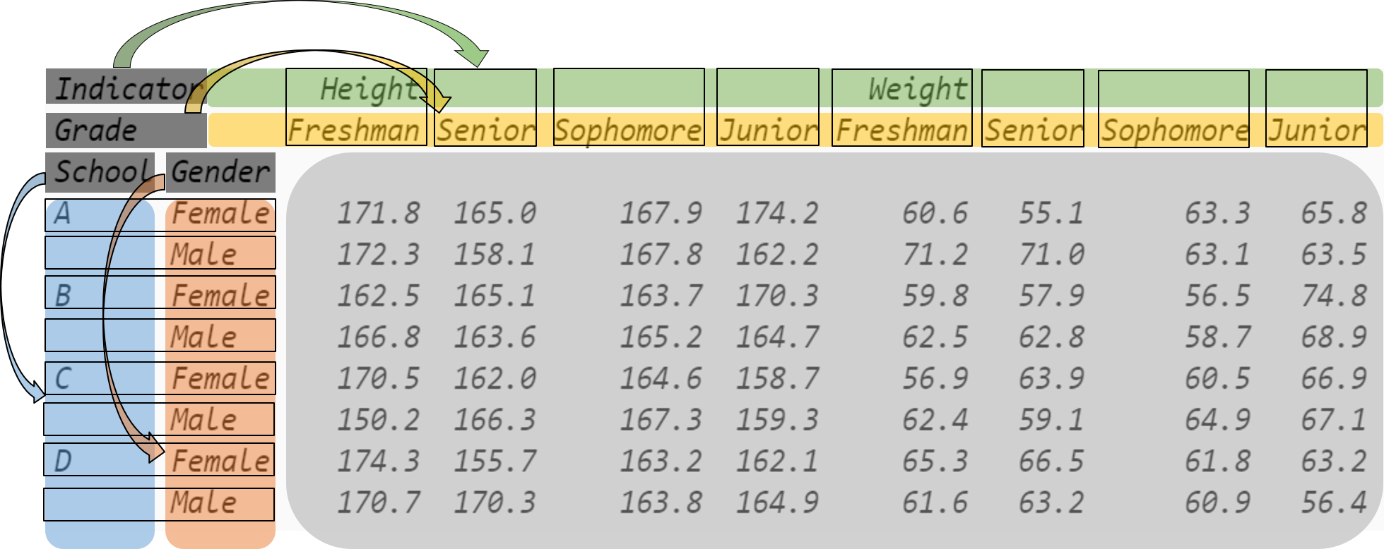
Like a single-level index, a MultiIndex has names: in the figure, School and Gender are the names of the first and second row-index levels, while Indicator and Grade name the first and second column-index levels.
The names and values of an index can be obtained through the names and values attributes, respectively:
| |
FrozenList(['School', 'Gender'])
| |
FrozenList(['Indicator', 'Grade'])
| |
array([('A', 'Female'), ('A', 'Male'), ('B', 'Female'), ('B', 'Male'),
       ('C', 'Female'), ('C', 'Male'), ('D', 'Female'), ('D', 'Male')],
      dtype=object)
| |
array([('Height', 'Freshman'), ('Height', 'Senior'),
       ('Height', 'Sophomore'), ('Height', 'Junior'),
       ('Weight', 'Freshman'), ('Weight', 'Senior'),
       ('Weight', 'Sophomore'), ('Weight', 'Junior')], dtype=object)
To obtain the index of a single level, use get_level_values:
| |
Index(['A', 'A', 'B', 'B', 'C', 'C', 'D', 'D'], dtype='object', name='School')
For indexes—whether single-level or multi-level—users cannot modify an element via index_obj[0] = item, nor rename a level via index_name[0] = new_name. How to change these attributes is discussed in Section 3.
2. The loc indexer with multi-level indexes
With the structure in mind, let us return to the original table and set school and grade as the index. The rows now form a multi-level index while the columns remain single-level; because the default column index has no name, there are no names in the slots corresponding to Indicator and Grade in the figure above.
| |
| Name | Gender | Weight | Transfer | ||
|---|---|---|---|---|---|
| School | Grade | ||||
| Shanghai Jiao Tong University | Freshman | Gaopeng Yang | Female | 46.0 | N |
| Peking University | Freshman | Changqiang You | Male | 70.0 | N |
| Shanghai Jiao Tong University | Senior | Mei Sun | Male | 89.0 | N |
| Fudan University | Sophomore | Xiaojuan Sun | Female | 41.0 | N |
| Sophomore | Gaojuan You | Male | 74.0 | N |
Because a single element of a multi-index is a tuple, the loc and iloc methods introduced in Section 1 carry over directly: simply replace the scalar with the corresponding tuple.
When passing a list of tuples, a single tuple, or a function returning either, sort the index first to avoid a performance warning:
| |
pandas.errors.PerformanceWarning('indexing past lexsort depth may impact performance.')
| |
| Name | Gender | Weight | Transfer | ||
|---|---|---|---|---|---|
| School | Grade | ||||
| Fudan University | Junior | Yanli You | Female | 48.0 | N |
| Junior | Chunqiang Chu | Male | 72.0 | N | |
| Junior | Changfeng Lv | Male | 76.0 | N | |
| Junior | Yanjuan Lv | Female | 49.0 | NaN | |
| Junior | Gaoqiang Zhou | Female | 43.0 | N |
| |
| Name | Gender | Weight | Transfer | ||
|---|---|---|---|---|---|
| School | Grade | ||||
| Fudan University | Senior | Chengpeng Zheng | Female | 38.0 | N |
| Senior | Feng Zhou | Female | 47.0 | N | |
| Senior | Gaomei Lv | Female | 34.0 | N | |
| Senior | Chunli Lv | Female | 56.0 | N | |
| Senior | Chengpeng Zhou | Male | 81.0 | N |
| |
| Name | Gender | Weight | Transfer | ||
|---|---|---|---|---|---|
| School | Grade | ||||
| Fudan University | Freshman | Feng Wang | Male | 74.0 | N |
| Junior | Chunqiang Chu | Male | 72.0 | N | |
| Junior | Changfeng Lv | Male | 76.0 | N | |
| Senior | Chengpeng Zhou | Male | 81.0 | N | |
| Senior | Chengpeng Qian | Male | 73.0 | Y |
| |
| Name | Gender | Weight | Transfer | ||
|---|---|---|---|---|---|
| School | Grade | ||||
| Fudan University | Junior | Yanli You | Female | 48.0 | N |
| Junior | Chunqiang Chu | Male | 72.0 | N | |
| Junior | Changfeng Lv | Male | 76.0 | N | |
| Junior | Yanjuan Lv | Female | 49.0 | NaN | |
| Junior | Gaoqiang Zhou | Female | 43.0 | N |
A caveat about slicing: in a single-level index a slice works as long as the endpoint elements are unique, but with a multi-level index you must sort before slicing—whether or not the tuples are repeated in the index—or an error will be raised:
| |
pandas.errors.UnsortedIndexError('Key length (2) was greater than MultiIndex lexsort depth (0)')
| |
| Name | Gender | Weight | Transfer | ||
|---|---|---|---|---|---|
| School | Grade | ||||
| Fudan University | Senior | Chengpeng Zheng | Female | 38.0 | N |
| Senior | Feng Zhou | Female | 47.0 | N | |
| Senior | Gaomei Lv | Female | 34.0 | N | |
| Senior | Chunli Lv | Female | 56.0 | N | |
| Senior | Chengpeng Zhou | Male | 81.0 | N |
| |
| Name | Gender | Weight | Transfer | ||
|---|---|---|---|---|---|
| School | Grade | ||||
| Shanghai Jiao Tong University | Freshman | Gaopeng Yang | Female | 46.0 | N |
| Peking University | Freshman | Changqiang You | Male | 70.0 | N |
| Shanghai Jiao Tong University | Senior | Mei Sun | Male | 89.0 | N |
| Fudan University | Sophomore | Xiaojuan Sun | Female | 41.0 | N |
| Tsinghua University | Freshman | Xiaoli Qian | Female | 51.0 | N |
| |
pandas.errors.UnsortedIndexError('Key length (2) was greater than MultiIndex lexsort depth (0)')
| |
| Name | Gender | Weight | Transfer | ||
|---|---|---|---|---|---|
| School | Grade | ||||
| Fudan University | Senior | Chengpeng Zheng | Female | 38.0 | N |
| Sophomore | Xiaojuan Sun | Female | 41.0 | N | |
| Peking University | Freshman | Changqiang You | Male | 70.0 | N |
| Junior | Juan Xu | Female | NaN | N | |
| Senior | Changli Lv | Female | 41.0 | N |
Tuples in a multi-index also have a special use: they let you index by the cross-product of elements from several levels, provided you also specify the loc columns—use : to select them all. The elements chosen from each level are stored in a list, and the form passed to loc is [(level_0_list, level_1_list), cols]. For example, to obtain all sophomores and juniors from Peking University and Fudan University:
| |
| Name | Gender | Weight | Transfer | ||
|---|---|---|---|---|---|
| School | Grade | ||||
| Peking University | Sophomore | Changmei Xu | Female | 43.0 | N |
| Sophomore | Xiaopeng Qin | Male | NaN | N | |
| Sophomore | Mei Xu | Female | 39.0 | N | |
| Sophomore | Xiaoli Zhou | Female | 55.0 | N | |
| Sophomore | Peng Han | Female | 34.0 | NaN |
| |
(33, 4)
The next statement looks similar but still passes a list of elements (tuples, in this case), and it means something different: select juniors at Peking University together with sophomores at Fudan University:
| |
| Name | Gender | Weight | Transfer | ||
|---|---|---|---|---|---|
| School | Grade | ||||
| Peking University | Junior | Juan Xu | Female | NaN | N |
| Junior | Changjuan You | Female | 47.0 | N | |
| Junior | Gaoli Xu | Female | 48.0 | N | |
| Junior | Gaoquan Zhou | Male | 70.0 | N | |
| Junior | Qiang You | Female | 56.0 | N |
| |
(16, 4)
3. The IndexSlice object
The methods described earlier can slice only an entire tuple, even when the index has no duplicates; they cannot slice each level separately, nor mix a slice with a Boolean list. The IndexSlice object solves this problem. It has two forms—loc[idx[*,*]] and loc[idx[*,*],idx[*,*]]—which we introduce below. For demonstration, we construct a DataFrame with a non-duplicated index:
| |
| Big | D | E | F | |||||||
|---|---|---|---|---|---|---|---|---|---|---|
| Small | d | e | f | d | e | f | d | e | f | |
| Upper | Lower | |||||||||
| A | a | 3 | 6 | -9 | -6 | -6 | -2 | 0 | 9 | -5 |
| b | -3 | 3 | -8 | -3 | -2 | 5 | 8 | -4 | 4 | |
| c | -1 | 0 | 7 | -4 | 6 | 6 | -9 | 9 | -6 | |
| B | a | 8 | 5 | -2 | -9 | -8 | 0 | -9 | 1 | -6 |
| b | 2 | 9 | -7 | -9 | -9 | -5 | -4 | -3 | -1 | |
| c | 8 | 6 | -5 | 0 | 1 | -8 | -8 | -2 | 0 | |
| C | a | -6 | -3 | 2 | 5 | 9 | -9 | 5 | -6 | 3 |
| b | 1 | 2 | -5 | -3 | -5 | 6 | -6 | 3 | -5 | |
| c | -1 | 5 | 6 | -6 | 6 | 4 | 7 | 8 | -4 | |
To use the silce object, you must define it first:
| |
[a] The loc[idx[*,*]] form
This form cannot slice different levels separately. The first * selects rows and the second selects columns, much like plain loc:
| |
| Big | D | E | F | |||||
|---|---|---|---|---|---|---|---|---|
| Small | f | d | e | f | d | e | f | |
| Upper | Lower | |||||||
| C | a | 2 | 5 | 9 | -9 | 5 | -6 | 3 |
| b | -5 | -3 | -5 | 6 | -6 | 3 | -5 | |
| c | 6 | -6 | 6 | 4 | 7 | 8 | -4 | |
Indexing with a Boolean series is also supported:
| |
| Big | D | F | ||
|---|---|---|---|---|
| Small | d | e | e | |
| Upper | Lower | |||
| A | a | 3 | 6 | 9 |
| b | -3 | 3 | -4 | |
| c | -1 | 0 | 9 | |
[b] The loc[idx[*,*],idx[*,*]] form
This form can slice level by level: the first idx refers to the row index, the second to the column index.
| |
| Big | E | F | |||
|---|---|---|---|---|---|
| Small | e | f | e | f | |
| Upper | Lower | ||||
| A | b | -2 | 5 | -4 | 4 |
| c | 6 | 6 | 9 | -6 | |
One restriction, however: functions are not supported in this form:
| |
KeyError(<function __main__.<lambda>(x)>)
4. Constructing multi-level indexes
We have seen the structure of multi-indexed tables and how to slice them. Beyond set_index, how can you build a multi-index yourself? Three common methods are from_tuples, from_arrays, from_product, all of them functions on the pd.MultiIndex object.
from_tuples builds an index from a supplied list of tuples:
| |
MultiIndex([('a', 'cat'),
            ('a', 'dog'),
            ('b', 'cat'),
            ('b', 'dog')],
           names=['First', 'Second'])
from_arrays builds an index from the lists corresponding to each level in the supplied list:
| |
MultiIndex([('a', 'cat'),
            ('a', 'dog'),
            ('b', 'cat'),
            ('b', 'dog')],
           names=['First', 'Second'])
from_product builds an index from the Cartesian product of the given lists:
| |
MultiIndex([('a', 'cat'),
            ('a', 'dog'),
            ('b', 'cat'),
            ('b', 'dog')],
           names=['First', 'Second'])
III. Common index operations
1. Swapping and dropping index levels
To make the swapping process easier to follow, here is an example with a three-level index:
| |
| Big | C | D | ||||||||
|---|---|---|---|---|---|---|---|---|---|---|
| Small | c | d | c | d | ||||||
| Other | cat | dog | cat | dog | cat | dog | cat | dog | ||
| Upper | Lower | Extra | ||||||||
| A | a | alpha | 3 | 6 | -9 | -6 | -6 | -2 | 0 | 9 |
| beta | -5 | -3 | 3 | -8 | -3 | -2 | 5 | 8 | ||
| b | alpha | -4 | 4 | -1 | 0 | 7 | -4 | 6 | 6 | |
| beta | -9 | 9 | -6 | 8 | 5 | -2 | -9 | -8 | ||
| B | a | alpha | 0 | -9 | 1 | -6 | 2 | 9 | -7 | -9 |
| beta | -9 | -5 | -4 | -3 | -1 | 8 | 6 | -5 | ||
| b | alpha | 0 | 1 | -8 | -8 | -2 | 0 | -6 | -3 | |
| beta | 2 | 5 | 9 | -9 | 5 | -6 | 3 | 1 | ||
Index levels are swapped with swaplevel and reorder_levels. The former can exchange only two levels, whereas the latter rearranges any number; both let you specify the axis—row index or column index—on which to operate:
| |
| Other | cat | dog | cat | dog | cat | dog | cat | dog | ||
|---|---|---|---|---|---|---|---|---|---|---|
| Small | c | c | d | d | c | c | d | d | ||
| Big | C | C | C | C | D | D | D | D | ||
| Upper | Lower | Extra | ||||||||
| A | a | alpha | 3 | 6 | -9 | -6 | -6 | -2 | 0 | 9 |
| beta | -5 | -3 | 3 | -8 | -3 | -2 | 5 | 8 | ||
| b | alpha | -4 | 4 | -1 | 0 | 7 | -4 | 6 | 6 | |
| beta | -9 | 9 | -6 | 8 | 5 | -2 | -9 | -8 | ||
| B | a | alpha | 0 | -9 | 1 | -6 | 2 | 9 | -7 | -9 |
| |
| Big | C | D | ||||||||
|---|---|---|---|---|---|---|---|---|---|---|
| Small | c | d | c | d | ||||||
| Other | cat | dog | cat | dog | cat | dog | cat | dog | ||
| Extra | Upper | Lower | ||||||||
| alpha | A | a | 3 | 6 | -9 | -6 | -6 | -2 | 0 | 9 |
| beta | A | a | -5 | -3 | 3 | -8 | -3 | -2 | 5 | 8 |
| alpha | A | b | -4 | 4 | -1 | 0 | 7 | -4 | 6 | 6 |
| beta | A | b | -9 | 9 | -6 | 8 | 5 | -2 | -9 | -8 |
| alpha | B | a | 0 | -9 | 1 | -6 | 2 | 9 | -7 | -9 |
[NOTE] Swapping indexes between axes
Here we only swap levels within the row or column index; swapping between indexes of different axes is discussed in Chapter 5.
[END]
To remove an index level, use the droplevel method:
| |
| Big | C | D | ||||||||
|---|---|---|---|---|---|---|---|---|---|---|
| Other | cat | dog | cat | dog | cat | dog | cat | dog | ||
| Upper | Lower | Extra | ||||||||
| A | a | alpha | 3 | 6 | -9 | -6 | -6 | -2 | 0 | 9 |
| beta | -5 | -3 | 3 | -8 | -3 | -2 | 5 | 8 | ||
| b | alpha | -4 | 4 | -1 | 0 | 7 | -4 | 6 | 6 | |
| beta | -9 | 9 | -6 | 8 | 5 | -2 | -9 | -8 | ||
| B | a | alpha | 0 | -9 | 1 | -6 | 2 | 9 | -7 | -9 |
| beta | -9 | -5 | -4 | -3 | -1 | 8 | 6 | -5 | ||
| b | alpha | 0 | 1 | -8 | -8 | -2 | 0 | -6 | -3 | |
| beta | 2 | 5 | 9 | -9 | 5 | -6 | 3 | 1 | ||
| |
| Big | C | D | ||||||
|---|---|---|---|---|---|---|---|---|
| Small | c | d | c | d | ||||
| Other | cat | dog | cat | dog | cat | dog | cat | dog |
| Extra | ||||||||
| alpha | 3 | 6 | -9 | -6 | -6 | -2 | 0 | 9 |
| beta | -5 | -3 | 3 | -8 | -3 | -2 | 5 | 8 |
| alpha | -4 | 4 | -1 | 0 | 7 | -4 | 6 | 6 |
| beta | -9 | 9 | -6 | 8 | 5 | -2 | -9 | -8 |
| alpha | 0 | -9 | 1 | -6 | 2 | 9 | -7 | -9 |
| beta | -9 | -5 | -4 | -3 | -1 | 8 | 6 | -5 |
| alpha | 0 | 1 | -8 | -8 | -2 | 0 | -6 | -3 |
| beta | 2 | 5 | 9 | -9 | 5 | -6 | 3 | 1 |
2. Modifying index attributes
The names of index levels can be changed with rename_axis, most commonly by passing a dictionary mapping old names to new ones:
| |
| Big | C | D | ||||||||
|---|---|---|---|---|---|---|---|---|---|---|
| Small | c | d | c | d | ||||||
| Changed_Col | cat | dog | cat | dog | cat | dog | cat | dog | ||
| Changed_row | Lower | Extra | ||||||||
| A | a | alpha | 3 | 6 | -9 | -6 | -6 | -2 | 0 | 9 |
| beta | -5 | -3 | 3 | -8 | -3 | -2 | 5 | 8 | ||
| b | alpha | -4 | 4 | -1 | 0 | 7 | -4 | 6 | 6 | |
| beta | -9 | 9 | -6 | 8 | 5 | -2 | -9 | -8 | ||
| B | a | alpha | 0 | -9 | 1 | -6 | 2 | 9 | -7 | -9 |
The rename method changes index values; with a multi-index you need to specify the level number via level:
| |
| Big | C | D | ||||||||
|---|---|---|---|---|---|---|---|---|---|---|
| Small | c | d | c | d | ||||||
| Other | not_cat | dog | not_cat | dog | not_cat | dog | not_cat | dog | ||
| Upper | Lower | Extra | ||||||||
| A | a | alpha | 3 | 6 | -9 | -6 | -6 | -2 | 0 | 9 |
| beta | -5 | -3 | 3 | -8 | -3 | -2 | 5 | 8 | ||
| b | alpha | -4 | 4 | -1 | 0 | 7 | -4 | 6 | 6 | |
| beta | -9 | 9 | -6 | 8 | 5 | -2 | -9 | -8 | ||
| B | a | alpha | 0 | -9 | 1 | -6 | 2 | 9 | -7 | -9 |
The argument can also be a function whose input is the index element:
| |
| Big | C | D | ||||||||
|---|---|---|---|---|---|---|---|---|---|---|
| Small | c | d | c | d | ||||||
| Other | cat | dog | cat | dog | cat | dog | cat | dog | ||
| Upper | Lower | Extra | ||||||||
| A | a | ALPHA | 3 | 6 | -9 | -6 | -6 | -2 | 0 | 9 |
| BETA | -5 | -3 | 3 | -8 | -3 | -2 | 5 | 8 | ||
| b | ALPHA | -4 | 4 | -1 | 0 | 7 | -4 | 6 | 6 | |
| BETA | -9 | 9 | -6 | 8 | 5 | -2 | -9 | -8 | ||
| B | a | ALPHA | 0 | -9 | 1 | -6 | 2 | 9 | -7 | -9 |
[Practice]
Try using a function inside rename_axis to accomplish the same task as the example—that is, replace Upper and Other with Changed_row and Changed_col, respectively.
[END]
Replacing every element of an index can be done with an iterator:
| |
| Big | C | D | ||||||||
|---|---|---|---|---|---|---|---|---|---|---|
| Small | c | d | c | d | ||||||
| Other | cat | dog | cat | dog | cat | dog | cat | dog | ||
| Upper | Lower | Extra | ||||||||
| A | a | a | 3 | 6 | -9 | -6 | -6 | -2 | 0 | 9 |
| b | -5 | -3 | 3 | -8 | -3 | -2 | 5 | 8 | ||
| b | c | -4 | 4 | -1 | 0 | 7 | -4 | 6 | 6 | |
| d | -9 | 9 | -6 | 8 | 5 | -2 | -9 | -8 | ||
| B | a | e | 0 | -9 | 1 | -6 | 2 | 9 | -7 | -9 |
| f | -9 | -5 | -4 | -3 | -1 | 8 | 6 | -5 | ||
| b | g | 0 | 1 | -8 | -8 | -2 | 0 | -6 | -3 | |
| h | 2 | 5 | 9 | -9 | 5 | -6 | 3 | 1 | ||
Modifying the element at a particular position is straightforward with a single-level index: fetch the index’s values attribute, edit the resulting list, and assign it back to the index object. With a multi-index, though, things get trickier. One solution is to temporarily move one level into the table as a column, make the changes, and then set it as the index again—operations covered in the next section.
Another function worth introducing is map, a method defined on Index. It resembles the functional form of rename seen above, except that instead of a level’s scalar value it receives the whole index tuple, which gives users a way to modify across levels. For example, the uppercase conversion above can be written equivalently as:
| |
| Big | C | D | ||||||||
|---|---|---|---|---|---|---|---|---|---|---|
| Small | c | d | c | d | ||||||
| Other | cat | dog | cat | dog | cat | dog | cat | dog | ||
| Upper | Lower | Extra | ||||||||
| A | a | ALPHA | 3 | 6 | -9 | -6 | -6 | -2 | 0 | 9 |
| BETA | -5 | -3 | 3 | -8 | -3 | -2 | 5 | 8 | ||
| b | ALPHA | -4 | 4 | -1 | 0 | 7 | -4 | 6 | 6 | |
| BETA | -9 | 9 | -6 | 8 | 5 | -2 | -9 | -8 | ||
| B | a | ALPHA | 0 | -9 | 1 | -6 | 2 | 9 | -7 | -9 |
Another use of map is compressing a multi-index, which is helpful in some operations in Chapters 4 and 5:
| |
| Big | C | D | ||||||
|---|---|---|---|---|---|---|---|---|
| Small | c | d | c | d | ||||
| Other | cat | dog | cat | dog | cat | dog | cat | dog |
| A-a-alpha | 3 | 6 | -9 | -6 | -6 | -2 | 0 | 9 |
| A-a-beta | -5 | -3 | 3 | -8 | -3 | -2 | 5 | 8 |
| A-b-alpha | -4 | 4 | -1 | 0 | 7 | -4 | 6 | 6 |
| A-b-beta | -9 | 9 | -6 | 8 | 5 | -2 | -9 | -8 |
| B-a-alpha | 0 | -9 | 1 | -6 | 2 | 9 | -7 | -9 |
The process can also be reversed to expand the index:
| |
| Big | C | D | ||||||||
|---|---|---|---|---|---|---|---|---|---|---|
| Small | c | d | c | d | ||||||
| Other | cat | dog | cat | dog | cat | dog | cat | dog | ||
| A | a | alpha | 3 | 6 | -9 | -6 | -6 | -2 | 0 | 9 |
| beta | -5 | -3 | 3 | -8 | -3 | -2 | 5 | 8 | ||
| b | alpha | -4 | 4 | -1 | 0 | 7 | -4 | 6 | 6 | |
| beta | -9 | 9 | -6 | 8 | 5 | -2 | -9 | -8 | ||
| B | a | alpha | 0 | -9 | 1 | -6 | 2 | 9 | -7 | -9 |
3. Setting and resetting the index
To illustrate the functions in this section, we construct a new table:
| |
| A | B | C | |
|---|---|---|---|
| 0 | a | P | 1 |
| 1 | a | Q | 2 |
| 2 | c | R | 3 |
| 3 | d | T | 4 |
An index is set with set_index, whose main parameter here is append: it indicates whether to keep the original index and add the new one as an inner level:
| |
| B | C | |
|---|---|---|
| A | ||
| a | P | 1 |
| a | Q | 2 |
| c | R | 3 |
| d | T | 4 |
| |
| B | C | ||
|---|---|---|---|
| A | |||
| 0 | a | P | 1 |
| 1 | a | Q | 2 |
| 2 | c | R | 3 |
| 3 | d | T | 4 |
Several columns can be designated as the index at once:
| |
| C | ||
|---|---|---|
| A | B | |
| a | P | 1 |
| Q | 2 | |
| c | R | 3 |
| d | T | 4 |
If the column you want to use as an index is not present in the table, you can pass the corresponding Series directly as an argument:
| |
| B | C | ||
|---|---|---|---|
| A | D | ||
| a | W | P | 1 |
| X | Q | 2 | |
| c | Y | R | 3 |
| d | Z | T | 4 |
reset_index is the inverse of set_index. Its main parameter, drop, decides whether the removed index level is discarded instead of being added back as a column:
| |
| D | B | C | |
|---|---|---|---|
| A | |||
| a | W | P | 1 |
| a | X | Q | 2 |
| c | Y | R | 3 |
| d | Z | T | 4 |
| |
| B | C | |
|---|---|---|
| A | ||
| a | P | 1 |
| a | Q | 2 |
| c | R | 3 |
| d | T | 4 |
If you reset every index, pandas simply generates a fresh default index:
| |
| A | D | B | C | |
|---|---|---|---|---|
| 0 | a | W | P | 1 |
| 1 | a | X | Q | 2 |
| 2 | c | Y | R | 3 |
| 3 | d | Z | T | 4 |
4. Reshaping the index
On some occasions you need to expand or trim an index. More precisely, given a new index, you fill a table built on that index with the elements associated with the corresponding labels in the original table. For example, the table below holds employee information; we want to build a new table that adds one employee while dropping the height column and adding a gender column:
| |
| Weight | Height | |
|---|---|---|
| 1001 | 60 | 176 |
| 1003 | 70 | 180 |
| 1002 | 80 | 179 |
| |
| Weight | Gender | |
|---|---|---|
| 1001 | 60.0 | NaN |
| 1002 | 80.0 | NaN |
| 1003 | 70.0 | NaN |
| 1004 | NaN | NaN |
Such needs arise frequently when filling in time points of a time-series index or extending ID numbering. Also note that data from the old table and the new one are aligned automatically by index. Even if, say, ID 1002 came after ID 1003 in the original table but the order is reversed in the new one, reindex matches elements by label, regardless of position.
A function similar to reindex is reindex_like, which reshapes the called table’s index to match the index of the table passed in. If a table with the desired index already exists, the previous operation can be written as follows:
| |
| Weight | Gender | |
|---|---|---|
| 1001 | 60.0 | NaN |
| 1002 | 80.0 | NaN |
| 1003 | 70.0 | NaN |
| 1004 | NaN | NaN |
IV. Index arithmetic
1. Rules of set operations
It is often useful to retrieve rows satisfying a condition by means of set operations. Suppose two tables A and B are both indexed by employee number and you want all employees whose IDs lie in the intersection of the two indexes; operations on Index make this easy.
Before that, let us review the four common set operations:
$$\rm S_A.intersection(S_B) = \rm S_A \cap S_B \Leftrightarrow \rm \{x|x\in S_A\, and\, x\in S_B\}$$$$\rm S_A.union(S_B) = \rm S_A \cup S_B \Leftrightarrow \rm \{x|x\in S_A\, or\, x\in S_B\}$$$$\rm S_A.difference(S_B) = \rm S_A - S_B \Leftrightarrow \rm \{x|x\in S_A\, and\, x\notin S_B\}$$$$\rm S_A.symmetric\_difference(S_B) = \rm S_A\triangle S_B\Leftrightarrow \rm \{x|x\in S_A\cup S_B - S_A\cap S_B\}$$2. General index operations
Because the elements of a set are distinct whereas an index may contain duplicates, call unique first to remove duplicates before performing the operation. Two of the simplest example tables follow:
| |
Index(['b'], dtype='object')
| |
Index(['a', 'b', 'c'], dtype='object')
| |
Index(['a'], dtype='object')
| |
Index(['a', 'c'], dtype='object')
If the columns to be used in a set operation are not set as the index, one approach is to convert them to an index, perform the operation, and then restore them; another is to use isin. For example, select the rows whose id values lie in the intersection from the first table after resetting its index:
| |
| id1 | 0 | 1 | |
|---|---|---|---|
| 0 | a | 0 | 1 |
| 1 | b | 1 | 2 |
| 2 | a | 3 | 4 |
| |
| id2 | 0 | 1 | |
|---|---|---|---|
| 0 | b | 4 | 5 |
| 1 | b | 2 | 6 |
| 2 | c | 7 | 1 |
| |
| id1 | 0 | 1 | |
|---|---|---|---|
| 1 | b | 1 | 2 |
V. Exercises
Ex1: Company employee dataset
Here is a dataset of company employees:
| |
| EmployeeID | birthdate_key | age | city_name | department | job_title | gender | |
|---|---|---|---|---|---|---|---|
| 0 | 1318 | 1/3/1954 | 61 | Vancouver | Executive | CEO | M |
| 1 | 1319 | 1/3/1957 | 58 | Vancouver | Executive | VP Stores | F |
| 2 | 1320 | 1/2/1955 | 60 | Vancouver | Executive | Legal Counsel | F |
- Using only
queryand, separately, onlyloc, select male employees aged forty or under who work in theDairyorBakerydepartment. - Select the 1st, 3rd, and second-to-last columns of the rows whose employee
IDis odd. - Carry out the following index operations in order:
- Set the last three columns as the index, then swap the inner and outer levels
- Restore the middle index level
- Rename the outer level to
Gender - Join the two row-index levels with an underscore
- Split the row index back into its original state
- Rename the index to the name of the original table
- Restore the default index while keeping the columns in their original relative positions
Ex2: Chocolate dataset
Here is a dataset of chocolate ratings:
| |
| Company | Review\r\nDate | Cocoa\r\nPercent | Company\r\nLocation | Rating | |
|---|---|---|---|---|---|
| 0 | A. Morin | 2016 | 63% | France | 3.75 |
| 1 | A. Morin | 2015 | 70% | France | 2.75 |
| 2 | A. Morin | 2015 | 70% | France | 3.00 |
- Replace the
\nin the column index names with spaces. - Chocolate
Ratingscores range from 1 to 5 in steps of 0.25. Select the samples rated 2.75 or below whoseCocoa Percentis above the median. - After setting
Review DateandCompany Locationas the index, select samples whoseReview Dateis after 2012 and whoseCompany Locationis not amongFrance, Canada, Amsterdam, Belgium.