
Pandas Joining
| |
I. Relational Joins
1. Basic Concepts of Joins
Joining two related tables on one key or a set of keys is a common operation. For example, the score sheets for the various subjects of a student’s final exam can be joined on $\color{red}{\text{name}}$ and $\color{red}{\text{class}}$ into a single grade report; likewise, the various information tables of a company’s employees can be joined and summarized by $\color{red}{\text{employee ID}}$. As these examples show, in a relational join the $\color{red}{\text{key}}$ is of central importance and is usually specified with the on parameter.
Another essential element is the form of the join. In pandas, the relational join functions merge and join offer a how parameter that represents the join form: left join left, right join right, inner join inner, and outer join outer. Their differences are illustrated in the following diagram:
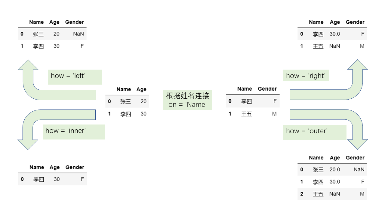
As the figure shows, a left join takes the keys of the left table as authoritative: if a key from the right table also exists in the left table, it is added to the left table; otherwise it is treated as a missing value. A right join is handled analogously. An inner join concerns itself only with keys that appear on both sides, whereas an outer join builds on the inner join by also including values present only on the left or only on the right — which is why the outer join is also called a full join.
In the simple example above, no key is repeated within a single table. What happens, then, when a key does repeat? A single rule covers it: any value appearing on both sides is combined by way of a Cartesian product, while a value appearing on only one side is handled according to the join form. The Cartesian product can be explained with a small example: suppose the key San Zhang occurs twice in the left table and twice in the right table. Matching the rows one by one produces a table that necessarily contains 2*2 rows with the name San Zhang. The diagram below shows a corresponding case:
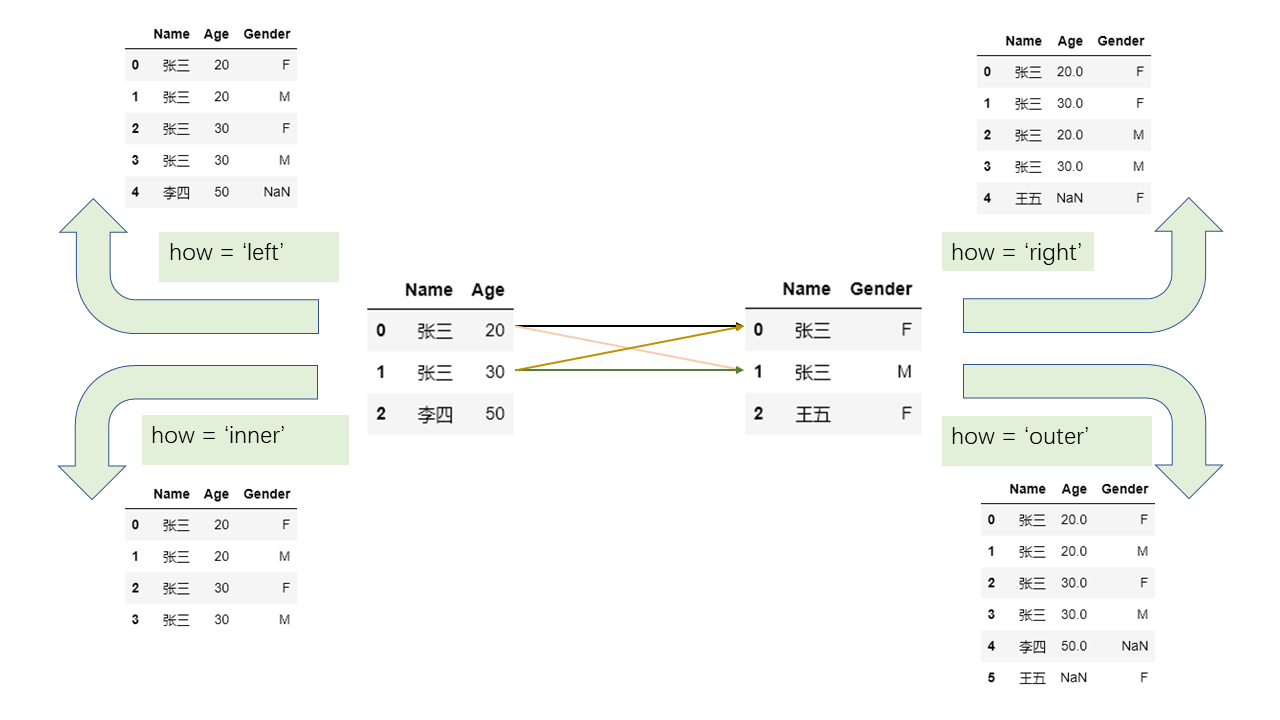
Different circumstances call for different join forms. Left and right joins are equivalent to each other; since the keys in their results are determined by one of the tables, they are often used to add information directionally to a target table. With inner and outer joins the two tables usually stand on an equal footing — swapping the left and right tables leaves the result unchanged — and the aim is to extract the intersection or the union of the keys. Which one to choose ultimately depends on the needs of the task at hand.
2. Value-Based Joins
In the illustrated example above, the two tables are joined on the values of one column. In fact, a join can also be based on a combination of several columns. Such value-based joins are implemented in pandas by the merge function; take the left join from the first figure, for instance:
| |
| Name | Age | Gender | |
|---|---|---|---|
| 0 | San Zhang | 20 | NaN |
| 1 | Si Li | 30 | F |
If the columns to be joined in the two tables do not share the same name, you can specify them through left_on and right_on:
| |
| df1_name | Age | df2_name | Gender | |
|---|---|---|---|---|
| 0 | San Zhang | 20 | NaN | NaN |
| 1 | Si Li | 30 | Si Li | F |
When duplicate column names occur in the two tables, the suffixes parameter comes into play. Suppose you are merging exam results, with the first table recording Chinese scores and the second recording math scores:
| |
| Name | Grade_Chinese | Grade_Math | |
|---|---|---|---|
| 0 | San Zhang | 70 | 80 |
Repeated elements can be troublesome on occasion. Consider two students from different classes who happen to share a name; in such a case you must pass several columns to on so that the join is carried out correctly:
| |
| Name | Age | Class | |
|---|---|---|---|
| 0 | San Zhang | 20 | one |
| 1 | San Zhang | 21 | two |
| |
| Name | Gender | Class | |
|---|---|---|---|
| 0 | San Zhang | F | two |
| 1 | San Zhang | M | one |
| |
| Name | Age | Class_x | Gender | Class_y | |
|---|---|---|---|---|---|
| 0 | San Zhang | 20 | one | F | two |
| 1 | San Zhang | 20 | one | M | one |
| 2 | San Zhang | 21 | two | F | two |
| 3 | San Zhang | 21 | two | M | one |
| |
| Name | Age | Class | Gender | |
|---|---|---|---|---|
| 0 | San Zhang | 20 | one | M |
| 1 | San Zhang | 21 | two | F |
The examples above show that a join relying on uniqueness breaks down when the keys are not unique. The example has only a handful of rows, but real data may involve hundreds of thousands or even millions of rows; to guarantee uniqueness there, besides checking for duplicates with duplicated, merge also offers a validate parameter that checks the uniqueness mode of the join. Three modes are available: one-to-one 1:1, one-to-many 1:m, and many-to-one m:1. The first means the keys are unique in both tables; the latter two mean the keys are unique in the left table and in the right table, respectively.
[Exercise]
In the multi-column key example above, the incorrect form is clearly a many-to-many join, whereas the correct form is a one-to-one join. Modify the original tables so that the correct multi-column form passes validate='1:m' but fails validate='m:1'.
[END]
3. Index Joins
An index join treats the index as the key, so in essence it is no different from a value join. In pandas, index joins are handled by the join function, which takes fewer options than merge. Apart from the mandatory on and how, you may specify left and right suffixes — lsuffix and rsuffix — for overlapping columns. Here on refers to the index name; with a single-level index, omitting the argument means joining on the current index.
| |
| Age | Gender | |
|---|---|---|
| Name | ||
| San Zhang | 20 | NaN |
| Si Li | 30 | F |
Following the example in subsection 2, write the join version that merges the Chinese and math scores:
| |
| Grade_Chinese | Grade_Math | |
|---|---|---|
| Name | ||
| San Zhang | 70 | 80 |
When you want join to do what merge does with several keys, a multi-level index is required. The last example with merge, for instance, can be written as follows:
| |
| Age | ||
|---|---|---|
| Name | Class | |
| San Zhang | one | 20 |
| two | 21 |
| |
| Gender | ||
|---|---|---|
| Name | Class | |
| San Zhang | two | F |
| one | M |
| |
| Age | Gender | ||
|---|---|---|---|
| Name | Class | ||
| San Zhang | one | 20 | M |
| two | 21 | F |
II. Directional Joins
1. concat
The previous section introduced relational joins, whose most important parameters are on and how. Sometimes, however, the user does not care which column serves as the key and simply wants to concatenate two or more tables vertically or horizontally. pandas provides the concat function for precisely this need.
In concat, three parameters are used most often: axis, join, keys. They denote, respectively, the direction of concatenation, the join form, and the names that indicate in the new table which old table each row came from. Note carefully that join and keys here have nothing to do with the join function and the notion of keys discussed earlier.
By default axis=0, which concatenates several tables vertically and is commonly used to stack multiple samples; axis=1 concatenates them horizontally and is typically used to combine multiple fields or features.
For example, vertically combine the person records from several tables:
| |
| Name | Age | |
|---|---|---|
| 0 | San Zhang | 20 |
| 1 | Si Li | 30 |
| 0 | Wu Wang | 40 |
Horizontally combine the fields from several tables:
| |
| Name | Age | Grade | Gender | |
|---|---|---|---|---|
| 0 | San Zhang | 20 | 80 | M |
| 1 | Si Li | 30 | 90 | F |
Although concat is a function for relational-style combining, it still joins on indexes. Vertical concatenation aligns on the column index: by default join=outer, which keeps all columns and sets absent values to missing, whereas join=inner keeps only the columns that appear in both tables. Horizontal concatenation aligns on the row index, with the join parameter set in much the same way.
| |
| Name | Age | Gender | |
|---|---|---|---|
| 0 | San Zhang | 20.0 | NaN |
| 1 | Si Li | 30.0 | NaN |
| 0 | Wu Wang | NaN | M |
| |
| Name | Age | Grade | |
|---|---|---|---|
| 0 | San Zhang | 20.0 | NaN |
| 1 | Si Li | 30.0 | 80.0 |
| 2 | NaN | NaN | 90.0 |
| |
| Name | Age | Grade | |
|---|---|---|---|
| 1 | Si Li | 30 | 80 |
Therefore, once you have decided on a direct, multi-table concatenation — especially a horizontal one — it is wise to call reset_index first to restore the default integer index. Doing so prevents the erroneous results caused by misaligned indexes and by the Cartesian product of duplicate indexes.
Finally, keys is useful in situations where several tables have been combined and you still want to know which original table each row of the new table came from. Passing keys creates a multi-level index that labels the source. For instance, if the first table holds students from Class One and the second holds students from Class Two, you can combine them as follows:
| |
| Name | Age | ||
|---|---|---|---|
| one | 0 | San Zhang | 20 |
| 1 | Si Li | 21 | |
| two | 0 | Wu Wang | 21 |
2. Combining Series with Tables
concat allows directional concatenation among several tables. To append a single Series to the end of the rows or the end of the columns of a table, use append and assign, respectively.
In append, if the original table uses the default integer index, ignore_index=True labels the index of the new Series automatically; otherwise you must give the Series a name attribute.
| |
| Name | Age | |
|---|---|---|
| 0 | San Zhang | 20 |
| 1 | Si Li | 21 |
| 2 | Wu Wang | 21 |
As for assign, although it can add a new column, the same effect is usually achieved with df['new_col'] = .... The drawback of using [] is that it modifies the original table in place, whereas assign returns a temporary copy:
| |
| Name | Age | Grade | |
|---|---|---|---|
| 0 | San Zhang | 20 | 80 |
| 1 | Si Li | 21 | 90 |
| |
| Name | Age | Grade | |
|---|---|---|---|
| 0 | San Zhang | 20 | 80 |
| 1 | Si Li | 21 | 90 |
III. Join-Like Operations
Besides the join functions described above, pandas also provides several functions that carry out certain operations on two tables. Here they are grouped together under the name join-like operations.
1. Comparison
compare is a new function introduced in version 1.1.0. It compares two tables or two Series and summarizes their differences:
| |
| Name | Class | |||
|---|---|---|---|---|
| self | other | self | other | |
| 1 | Si Li | Li Si | NaN | NaN |
| 2 | NaN | NaN | three | Three |
The result reports the rows and columns where the values differ; positions that are the same are filled with the missing value NaN. Here other and self refer to the argument table passed in and to the calling table itself, respectively.
To display the comparison of every element in the tables in full, set keep_shape=True:
| |
| Name | Age | Class | ||||
|---|---|---|---|---|---|---|
| self | other | self | other | self | other | |
| 0 | NaN | NaN | NaN | NaN | NaN | NaN |
| 1 | Si Li | Li Si | NaN | NaN | NaN | NaN |
| 2 | NaN | NaN | NaN | NaN | three | Three |
2. Combination
The combine function combines two tables according to a rule you supply, automatically aligning column indexes when it compares them. For the function passed in, the argument at each step is a pair of same-named Series taken from the two tables, and the columns are visited in the order of the union of their names. The example below therefore passes four groups of series, A,B,C,D, each group holding one series from the left table and one from the right. While column A is being compared, s2 denotes an entirely empty series, because that column does not exist in the called table; in addition, the index of the series from the first table is reindexed to the union of the two indexes. You can inspect the whole process by inserting suitable print statements into the function you pass in.
The following example selects the smaller element at each corresponding index position:
| |
| A | B | C | D | |
|---|---|---|---|---|
| 0 | NaN | NaN | NaN | NaN |
| 1 | NaN | 4.0 | 6.0 | NaN |
| 2 | NaN | NaN | NaN | NaN |
[Exercise]
Building on the code above, modify it so that the four positions in df2 which were not replaced by values from df1 keep their original values.
[END]
In addition, setting the overwrite parameter to False preserves the columns of $\color{red}{\text{the called table}}$ that do not appear in the argument table, keeping their values instead of overwriting them with missing ones:
| |
| A | B | C | D | |
|---|---|---|---|---|
| 0 | 1.0 | NaN | NaN | NaN |
| 1 | 2.0 | 4.0 | 6.0 | NaN |
| 2 | NaN | NaN | NaN | NaN |
[Exercise]
Besides combine, pandas has a combine_first method: when two tables are combined, a missing value in the first table is filled with the value at the same index position in the second table. An example is given below; use combine to achieve the same result.
[END]
| |
| A | B | |
|---|---|---|
| 0 | 1.0 | 3.0 |
| 1 | 2.0 | 7.0 |
| 2 | 6.0 | 8.0 |
IV. Exercises
Ex1: The U.S. COVID-19 Dataset
We have a set of U.S. COVID-19 reports covering April 12 through November 16 (in the /data/us_report folder). Merge the Confirmed, Deaths, Recovered, Active figures for New York into a single table, indexed by a sequence of date strings generated as follows:
| |
['04-12-2020', '04-13-2020', '04-14-2020', '04-15-2020', '04-16-2020']
Ex2: Implementing the join Function
Implement a join function with a how parameter:
- Assume the two tables being joined have no columns in common.
- Call it as
join(df1, df2, how="left"). - Provide test cases.