
Pandas Handling Missing Data
| |
I. Counting and Deleting Missing Values
1. Counting Missing Information
Missing data can be examined with isna or isnull (the two functions are interchangeable) to see whether each cell is missing; combined with mean, this yields the proportion of missing values in each column:
| |
| Grade | Name | Gender | Height | Weight | Transfer | |
|---|---|---|---|---|---|---|
| 0 | False | False | False | False | False | False |
| 1 | False | False | False | False | False | False |
| 2 | False | False | False | False | False | False |
| 3 | False | False | False | True | False | False |
| 4 | False | False | False | False | False | False |
| |
Grade       0.000
Name        0.000
Gender      0.000
Height      0.085
Weight      0.055
Transfer    0.060
dtype: float64
To retrieve the rows where a given column is missing or not missing, use boolean indexing with isna or notna on the Series. For example, to view the rows with a missing height:
| |
| Grade | Name | Gender | Height | Weight | Transfer | |
|---|---|---|---|---|---|---|
| 3 | Sophomore | Xiaojuan Sun | Female | NaN | 41.0 | N |
| 12 | Senior | Peng You | Female | NaN | 48.0 | NaN |
| 26 | Junior | Yanli You | Female | NaN | 48.0 | N |
| 36 | Freshman | Xiaojuan Qin | Male | NaN | 79.0 | Y |
| 60 | Freshman | Yanpeng Lv | Male | NaN | 65.0 | N |
To search across several columns at once — for rows that are all missing, have at least one missing value, or have none — combine isna, notna with any, all. For example, here are the three searches applied to the columns for height, weight, and transfer status:
| |
| Grade | Name | Gender | Height | Weight | Transfer | |
|---|---|---|---|---|---|---|
| 102 | Junior | Chengli Zhao | Male | NaN | NaN | NaN |
| |
| Grade | Name | Gender | Height | Weight | Transfer | |
|---|---|---|---|---|---|---|
| 3 | Sophomore | Xiaojuan Sun | Female | NaN | 41.0 | N |
| 9 | Junior | Juan Xu | Female | 164.8 | NaN | N |
| 12 | Senior | Peng You | Female | NaN | 48.0 | NaN |
| 21 | Senior | Xiaopeng Shen | Male | 166.0 | 62.0 | NaN |
| 26 | Junior | Yanli You | Female | NaN | 48.0 | N |
| |
| Grade | Name | Gender | Height | Weight | Transfer | |
|---|---|---|---|---|---|---|
| 0 | Freshman | Gaopeng Yang | Female | 158.9 | 46.0 | N |
| 1 | Freshman | Changqiang You | Male | 166.5 | 70.0 | N |
| 2 | Senior | Mei Sun | Male | 188.9 | 89.0 | N |
| 4 | Sophomore | Gaojuan You | Male | 174.0 | 74.0 | N |
| 5 | Freshman | Xiaoli Qian | Female | 158.0 | 51.0 | N |
2. Deleting Missing Information
Data processing often calls for dropping row samples or column features according to the size, proportion, or other characteristics of their missing values. pandas provides the dropna function for this task.
The main parameters of dropna are the axis direction axis (default 0, meaning rows are removed), the removal mode how, the threshold thresh for the number of non-missing values (a dimension is dropped when $\color{red}{\text{the number of non-missing values}}$ fails to reach this count), and the optional deletion subset subset. For how, the choices are any and all.
For example, drop the rows where at least one of height and weight is missing:
| |
(174, 6)
For example, drop the columns with more than 15 missing values:
| |
| Grade | Name | Gender | Weight | Transfer | |
|---|---|---|---|---|---|
| 0 | Freshman | Gaopeng Yang | Female | 46.0 | N |
| 1 | Freshman | Changqiang You | Male | 70.0 | N |
| 2 | Senior | Mei Sun | Male | 89.0 | N |
| 3 | Sophomore | Xiaojuan Sun | Female | 41.0 | N |
| 4 | Sophomore | Gaojuan You | Male | 74.0 | N |
Of course, dropna is not the only way; the two operations above can also be accomplished with boolean indexing:
| |
(174, 6)
| |
| Grade | Name | Gender | Weight | Transfer | |
|---|---|---|---|---|---|
| 0 | Freshman | Gaopeng Yang | Female | 46.0 | N |
| 1 | Freshman | Changqiang You | Male | 70.0 | N |
| 2 | Senior | Mei Sun | Male | 89.0 | N |
| 3 | Sophomore | Xiaojuan Sun | Female | 41.0 | N |
| 4 | Sophomore | Gaojuan You | Male | 74.0 | N |
II. Filling Missing Values and Interpolation
1. Filling with fillna
Three parameters of fillna see frequent use: value, method, limit. Here value is the fill value, either a scalar or a dictionary mapping indexes to elements; method is the fill strategy, with ffill filling forward from the preceding element and bfill filling backward from the following one; and limit gives the maximum number of times consecutive missing values are filled.
Let us construct a simple Series to illustrate the usage:
| |
a    NaN
a    1.0
a    NaN
b    NaN
c    2.0
d    NaN
dtype: float64
| |
a    NaN
a    1.0
a    1.0
b    1.0
c    2.0
d    2.0
dtype: float64
| |
a    NaN
a    1.0
a    1.0
b    NaN
c    2.0
d    2.0
dtype: float64
| |
a    1.5
a    1.0
a    1.5
b    1.5
c    2.0
d    1.5
dtype: float64
| |
a    100.0
a      1.0
a    100.0
b      NaN
c      2.0
d    200.0
dtype: float64
Sometimes a more sensible fill requires grouping first. For example, fill missing heights with the mean height within each grade:
| |
0    158.900000
1    166.500000
2    188.900000
3    163.075862
4    174.000000
Name: Height, dtype: float64
[Exercise]
Fill the missing values of a series by the following rule: an isolated missing value is replaced by the mean of its neighbours, whereas consecutive missing values are left untouched; thus [1, NaN, 3, NaN, NaN] becomes [1, 2, 3, NaN, NaN] after filling. Implement this with fillna. (Hint: make use of the limit parameter.)
[END]
2. Interpolation Functions
The documentation for the interpolate function lists many interpolation methods, including a large number from Scipy. Because many of them rely on fairly involved mathematics, only three common and simple cases are discussed here: linear interpolation, nearest-neighbour interpolation, and index interpolation.
For interpolate, besides the method itself (which defaults to linear), two parameters resemble those of fillna: limit_direction governs the direction, while limit caps the number of consecutive missing values to interpolate. By default the direction is forward, analogous to ffill in fillna; to restrict interpolation backward or in both directions, pass backward or both.
| |
array([nan, nan, 1., nan, nan, nan, 2., nan, nan])
For example, under the default linear method, carry out backward and two-way limited interpolation, capping the run length at 1:
| |
array([ nan, 1. , 1. , nan, nan, 1.75, 2. , nan, nan])
| |
array([ nan, 1. , 1. , 1.25, nan, 1.75, 2. , 2. , nan])
The second common approach is nearest-neighbour imputation, in which a missing element takes the value of the nearest non-missing element:
| |
array([nan, nan, 1., 1., 1., 2., 2., nan, nan])
Finally, index interpolation performs linear interpolation according to the size of the index. To demonstrate it, construct an index with unequal spacing:
| |
0      0.0
1      NaN
10    10.0
dtype: float64
| |
0      0.0
1      5.0
10    10.0
dtype: float64
| |
0      0.0
1      1.0
10    10.0
dtype: float64
This method also works with timestamp indexes. Other topics concerning time series are discussed in Chapter 10; here is a simple example:
| |
2020-01-01     0.0
2020-01-02     NaN
2020-01-11    10.0
dtype: float64
| |
2020-01-01     0.0
2020-01-02     5.0
2020-01-11    10.0
dtype: float64
| |
2020-01-01     0.0
2020-01-02     1.0
2020-01-11    10.0
dtype: float64
[NOTE] A note on polynomial and spline interpolation
In interpolate, choosing the polynomial method calls scipy.interpolate.interp1d(*,*,kind=order) internally, which in turn calls make_interp_spline; it is therefore spline interpolation rather than a polynomial fit in the spirit of numpy’s polyfit. Choosing spline, by contrast, makes pandas call scipy.interpolate.UnivariateSpline instead of ordinary spline interpolation. The documentation on this part is rather muddled, and the design of these options is questionable. Whenever you use either method, take care to pick the interpolation that truly fits your needs.
[END]
III. Nullable Types
1. Missing Markers and Their Drawbacks
In python, a missing value is denoted by None, which equals only itself and is unequal to every other element:
| |
True
| |
False
| |
False
| |
False
In numpy, missing values are represented by np.nan, which is unequal not only to any other element but also to itself:
| |
False
| |
False
| |
False
It is worth noting that although comparing the elements of a series or table containing missing values returns False at the positions of np.nan, the equals function skips positions where both sides are missing and returns True outright:
| |
0     True
1    False
dtype: bool
| |
False
| |
True
For time-series objects, pandas uses pd.NaT to denote missing values; it serves the same purpose as np.nan (time-series objects and their construction are discussed in Chapter 10):
| |
TimedeltaIndex(['0 days 00:00:30', NaT], dtype='timedelta64[ns]', freq=None)
| |
DatetimeIndex(['2020-01-01', 'NaT'], dtype='datetime64[ns]', freq=None)
So why introduce pd.NaT for missing values in time objects, and what would be wrong with storing them as np.nan? In pandas you will encounter objects of type object, a catch-all type: if a Series holds elements of several different types, its dtype becomes object. For example, a list holding both integers and strings:
| |
0      1
1    two
dtype: object
The root of the NaT problem is that np.nan is itself a floating-point type. If floats and time types were stored together without a new built-in missing type, the result would be an ambiguous object type — plainly undesirable.
| |
float
Moreover, owing to the floating-point nature of np.nan, a missing value in an integer Series turns its dtype into float64, while a missing value in a boolean Series turns it into object rather than bool:
| |
dtype('float64')
| |
dtype('O')
For all these reasons, starting with version 1.0.0, pandas set out to design a new missing type, pd.NA, along with three Nullable Series types: Int, boolean, and string.
2. Properties of Nullable Types
Taken literally, Nullable means capable of holding nulls — the Series type is, as it were, unfazed by missing values. For example, a missing value stored in any of the three Nullable types above is converted to the built-in pd.NA:
| |
0    <NA>
1       1
dtype: Int64
| |
0    <NA>
1    True
dtype: boolean
| |
0      <NA>
1    my_str
dtype: string
In an Int Series, the result of an operation is kept as a Nullable type whenever possible:
| |
0    <NA>
1       1
dtype: Int64
| |
0    <NA>
1    True
dtype: boolean
| |
0    NaN
1    0.0
dtype: float64
For a boolean Series, behaviour differs from a bool Series in two main respects.
First, a boolean list containing missing values cannot serve as an indexer, whereas boolean treats missing values as False:
| |
0    a
dtype: object
Second, in logical operations bool always returns False at a missing position, whereas boolean returns a value depending on whether the logic can determine a unique result. What does “determine a unique result” mean? A simple example: in True | pd.NA the result is necessarily True whatever the missing value happens to be; in False | pd.NA the outcome varies with the value of the missing element, so pd.NA is returned; in False & pd.NA the result is necessarily False regardless of the missing value.
| |
0    True
1    <NA>
dtype: boolean
| |
0    True
1    True
dtype: boolean
| |
0    False
1     <NA>
dtype: boolean
The specific properties of the string type are discussed in the next chapter on textual data.
In practical data work, after reading in a dataset you can convert it to Nullable types up front with convert_dtypes:
| |
School          string
Grade           string
Name            string
Gender          string
Height         float64
Weight           Int64
Transfer        string
Test_Number      Int64
Test_Date       string
Time_Record     string
dtype: object
3. Computation and Grouping of Missing Data
When sum, prod are called and addition and multiplication are involved, missing data is treated as 0 and 1 respectively, leaving the original result unchanged:
| |
14.0
| |
120.0
Cumulative functions automatically skip the positions occupied by missing values:
| |
0     2.0
1     5.0
2     NaN
3     9.0
4    14.0
dtype: float64
For scalar operations, every result is missing (and pd.NA behaves in the same way) except np.nan ** 0 and 1 ** np.nan, which produce definite values. Furthermore, np.nan always returns False in comparisons, whereas pd.NA returns pd.NA:
| |
False
| |
<NA>
| |
False
| |
<NA>
| |
nan
| |
nan
| |
nan
| |
1.0
| |
1
| |
1.0
| |
1
One more point deserves attention: though diff, pct_change are similar in purpose, they handle missing values differently. The former marks every part involved in a missing calculation as missing, whereas the latter sets the missing position to a 0% rate of change:
| |
0    NaN
1    1.0
2    NaN
3    NaN
4    1.0
dtype: float64
| |
0         NaN
1    0.500000
2    0.000000
3    0.333333
4    0.250000
dtype: float64
For certain functions, missing values can be handled as a category. For example, groupby, get_dummies accept parameters that add a missing category:
| |
| category | value | |
|---|---|---|
| 0 | a | 1 |
| 1 | a | 3 |
| 2 | b | 5 |
| 3 | NaN | 7 |
| 4 | NaN | 9 |
| |
category
a      2
b      5
NaN    8
Name: value, dtype: int64
| |
| a | b | NaN | |
|---|---|---|---|
| 0 | 1 | 0 | 0 |
| 1 | 1 | 0 | 0 |
| 2 | 0 | 1 | 0 |
| 3 | 0 | 0 | 1 |
| 4 | 0 | 0 | 1 |
IV. Exercises
Ex1: Testing the Correlation Between Missing Values and the Label
| |
| X_1 | X_2 | y | |
|---|---|---|---|
| 0 | NaN | NaN | 0 |
| 1 | NaN | NaN | 0 |
| 2 | NaN | NaN | 0 |
| 3 | 43.0 | NaN | 0 |
| 4 | NaN | NaN | 0 |
| |
X_1    0.855
X_2    0.894
y      0.000
dtype: float64
| |
0    0.918
1    0.082
Name: y, dtype: float64
In fact, the presence or absence of a missing value is itself sometimes a feature, and in some settings it may be related to the sign of the label. In statistics, a chi-square test can tell us whether the occurrence of missingness and the sign of the label are associated. Four cases can be distinguished: a positive with the feature missing, a negative with the feature missing, a positive with the feature present, and a negative with the feature present; let their sample counts be $n_{11}, n_{10}, n_{01}, n_{00}$, respectively. If the two were independent, the theoretical count of positives among the missing-feature cases should be close to the total number of missing-feature cases $\times$ the overall proportion of positives, namely:
$$E_{11} = n_{11} \approx (n_{11}+n_{10})\times\frac{n_{11}+n_{01}}{n_{11}+n_{10}+n_{01}+n_{00}} = F_{11}$$The other three cases follow the same reasoning. Write the actual and theoretical values as $E_{ij}, F_{ij}$, respectively; we would then like the statistic below to be as small as possible, since a small value means the observed counts lie close to those expected under independence:
$$S = \sum_{i\in \{0,1\}}\sum_{j\in \{0,1\}} \frac{(E_{ij}-F_{ij})^2}{F_{ij}}$$It can be shown that this statistic approximately follows a chi-square distribution with $1$ degree of freedom, i.e. $S\overset{\cdot}{\sim} \chi^2(1)$. The correlation can therefore be judged by computing $P(\chi^2(1)>S)$: when this probability falls below $0.05$, the missingness is regarded as related to the sign of the label — in other words, the theoretical value under independence differs markedly from the observed one.
The probability just mentioned is, for a $2\times2$ contingency table test in statistics, the $p$-value; it is available through scipy.stats.chi2.sf(S, 1). Using the material above, test the X_1, X_2 columns separately.
Ex2: Solving a Classification Problem with a Regression Model
KNN is a supervised learning model that handles both regression and classification. For a categorical variable, a KNN classifier can impute its missing values: measure the distance between the features of the missing sample and those of all the other samples; once n_neighbors=n is given, find the most frequent class among the $n$ nearest samples and assign it as the predicted class for the missing sample. The idea is illustrated below, where the unknown class is predicted to be yellow:
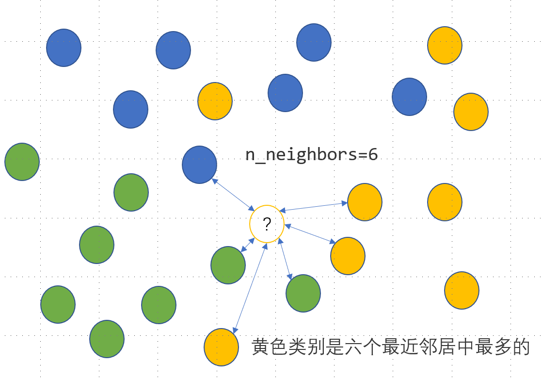
The feature data of the coloured points above are given below:
| |
| X1 | X2 | Color | |
|---|---|---|---|
| 0 | -2.5 | 2.8 | Blue |
| 1 | -1.5 | 1.8 | Blue |
| 2 | -0.8 | 2.8 | Blue |
Given the sample point to be predicted, $X_1=0.8, X_2=-0.2$, the predicted class can be written as follows:
| |
array(['Yellow'], dtype=object)
- For a regression problem the desired output is a concrete number, so the prediction comes from averaging the values of the nearest $n$ samples. Turn the classification problem above into a regression problem, using only
KNeighborsRegressorto reproduce whatKNeighborsClassifierdid. - Following the method in part 1, impute the missing values of the
Employmentvariable in theauditdataset.
| |
| ID | Age | Employment | Marital | Income | Gender | Hours | |
|---|---|---|---|---|---|---|---|
| 0 | 1004641 | 38 | Private | Unmarried | 81838.00 | Female | 72 |
| 1 | 1010229 | 35 | Private | Absent | 72099.00 | Male | 30 |
| 2 | 1024587 | 32 | Private | Divorced | 154676.74 | Male | 40 |