
Pandas Reshaping
| |
I. Reshaping Long and Wide Tables
What is a long table, and what is a wide table? The distinction is made with respect to a particular feature. If a table stores gender in one column, it is a long table with respect to gender; if gender is used as the column names and the cells hold values of some other related feature, the table is a wide table with respect to gender. The two tables below are, respectively, long and wide tables with respect to gender:
| |
| Gender | Height | |
|---|---|---|
| 0 | F | 163 |
| 1 | F | 160 |
| 2 | M | 175 |
| 3 | M | 180 |
| |
| Height: F | Height: M | |
|---|---|---|
| 0 | 163 | 175 |
| 1 | 160 | 180 |
Clearly the two tables carry exactly the same information - the same height figures - presented in different ways. That presentation depends chiefly on the layout chosen for the gender column: is it stored in the $\color{red}{\text{long}}$ form or the $\color{red}{\text{wide}}$ form? Accordingly, pandas provides a number of reshaping functions for this kind of long/wide conversion.
1. pivot
pivot is a typical function for turning a long table into a wide one. Consider the following example: the table stores the Chinese and math scores of San Zhang and Si Li, and we want those two subjects to appear as columns.
| |
| Class | Name | Subject | Grade | |
|---|---|---|---|---|
| 0 | 1 | San Zhang | Chinese | 80 |
| 1 | 1 | San Zhang | Math | 75 |
| 2 | 2 | Si Li | Chinese | 90 |
| 3 | 2 | Si Li | Math | 85 |
For a basic long-to-wide operation, three elements matter most: the row index of the reshaped table, the columns to be moved into the column index, and the values associated with those columns and rows. These correspond to the index, columns, and values parameters of pivot. The column index of the new table is the unique values of the columns columns, its row index is the unique values of the index columns, and values identifies the column holding the numbers to display.
| |
| Subject | Chinese | Math |
|---|---|---|
| Name | ||
| San Zhang | 80 | 75 |
| Si Li | 90 | 85 |
The color coding makes the reshaping process easier to follow:
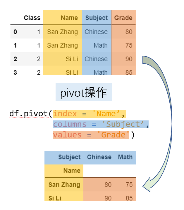
Using pivot requires a uniqueness condition: since each row-column pair in the new table maps to a single value, the row combinations of the index and columns columns in the original table must be unique. For example, changing San Zhang’s math score in the second row to Chinese would raise an error, because the pair ("San Zhang", "Chinese") would then occur twice for Name and Subject, leaving it unclear whether the reshaped cell should contain 80 or 75.
| |
ValueError('Index contains duplicate entries, cannot reshape')
Starting with pandas 1.1.0, all three pivot parameters may be set to lists, which means a multi-level index will be returned. Here is an example: the six columns below are class, name, examination type (midterm and final), subject, grade, and rank.
| |
| Class | Name | Examination | Subject | Grade | rank | |
|---|---|---|---|---|---|---|
| 0 | 1 | San Zhang | Mid | Chinese | 80 | 10 |
| 1 | 1 | San Zhang | Final | Chinese | 75 | 15 |
| 2 | 2 | Si Li | Mid | Chinese | 85 | 21 |
| 3 | 2 | Si Li | Final | Chinese | 65 | 15 |
| 4 | 1 | San Zhang | Mid | Math | 90 | 20 |
| 5 | 1 | San Zhang | Final | Math | 85 | 7 |
| 6 | 2 | Si Li | Mid | Math | 92 | 6 |
| 7 | 2 | Si Li | Final | Math | 88 | 2 |
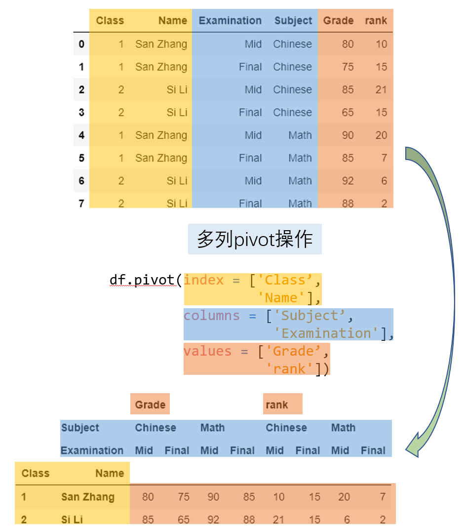
Now we want to move the four combinations formed by examination type and subject (midterm Chinese, final Chinese, midterm math, final math) into the column index, while reporting both grade and rank:
| |
| Grade | rank | ||||||||
|---|---|---|---|---|---|---|---|---|---|
| Subject | Chinese | Math | Chinese | Math | |||||
| Examination | Mid | Final | Mid | Final | Mid | Final | Mid | Final | |
| Class | Name | ||||||||
| 1 | San Zhang | 80 | 75 | 90 | 85 | 10 | 15 | 20 | 7 |
| 2 | Si Li | 85 | 65 | 92 | 88 | 21 | 15 | 6 | 2 |
By the uniqueness principle, the row index of the new table is equivalent to applying drop_duplicates to the columns in index, while the length of the column index equals the number of elements in values times the number of unique combinations in columns (computed just as for index). The diagram below makes the operation easy to grasp:
2. pivot_table
pivot relies on the uniqueness condition. When that condition fails, aggregation must collapse the multiple values sharing a row-column combination into one. Suppose San Zhang and Si Li each took two Chinese exams and two math exams, and the school’s rules make the final grade the average of the two scores; pivot alone cannot produce this result.
| |
| Name | Subject | Grade | |
|---|---|---|---|
| 0 | San Zhang | Chinese | 80 |
| 1 | San Zhang | Chinese | 90 |
| 2 | San Zhang | Math | 100 |
| 3 | San Zhang | Math | 90 |
| 4 | Si Li | Chinese | 70 |
| 5 | Si Li | Chinese | 80 |
| 6 | Si Li | Math | 85 |
| 7 | Si Li | Math | 95 |
pandas provides pivot_table for this purpose, where the aggfunc parameter is the aggregation function to use. The scenario above can be written as follows:
| |
| Subject | Chinese | Math |
|---|---|---|
| Name | ||
| San Zhang | 85 | 95 |
| Si Li | 75 | 90 |
The aggfunc argument accepts all the valid aggregation strings introduced in the previous chapter. You may also supply a custom function that takes a series and returns a scalar, which gives the same result equivalently:
| |
| Subject | Chinese | Math |
|---|---|---|
| Name | ||
| San Zhang | 85 | 95 |
| Si Li | 75 | 90 |
In addition, pivot_table can compute marginal summaries by setting margins=True; the aggregation applied at the margins matches the method given in aggfunc. The following table reports the mean Chinese and math scores, the mean scores of San Zhang and of Si Li, and the overall mean of all four scores:
| |
| Subject | Chinese | Math | All |
|---|---|---|---|
| Name | |||
| San Zhang | 85 | 95.0 | 90.00 |
| Si Li | 75 | 90.0 | 82.50 |
| All | 80 | 92.5 | 86.25 |
[Exercise]
In the marginal-summary example above, a row or column summary is the average of the corresponding row or column entries in the new table, while the grand total is the average of all four entries. Must this relationship always hold? If not, give an example to show why.
[END]
3. melt
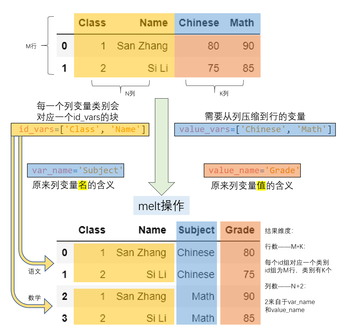
Long and wide tables differ only in presentation, not in the information they contain. Having used pivot to turn a long table into a wide one, we can reverse the operation to turn a wide table back into a long one; that is what melt does. In the example below, Subject is stored in the column index, and we want to compress it into a single column.
| |
| Class | Name | Chinese | Math | |
|---|---|---|---|---|
| 0 | 1 | San Zhang | 80 | 80 |
| 1 | 2 | Si Li | 90 | 75 |
| |
| Class | Name | Subject | Grade | |
|---|---|---|---|---|
| 0 | 1 | San Zhang | Chinese | 80 |
| 1 | 2 | Si Li | Chinese | 90 |
| 2 | 1 | San Zhang | Math | 80 |
| 3 | 2 | Si Li | Math | 75 |
The main parameters of melt and the compression process are illustrated below:
Since melt and pivot are inverse processes, we can of course use pivot to convert df_melted back into the form of df:
| |
| Subject | Chinese | Math | |
|---|---|---|---|
| Class | Name | ||
| 1 | San Zhang | 80 | 80 |
| 2 | Si Li | 90 | 75 |
| |
True
4. wide_to_long
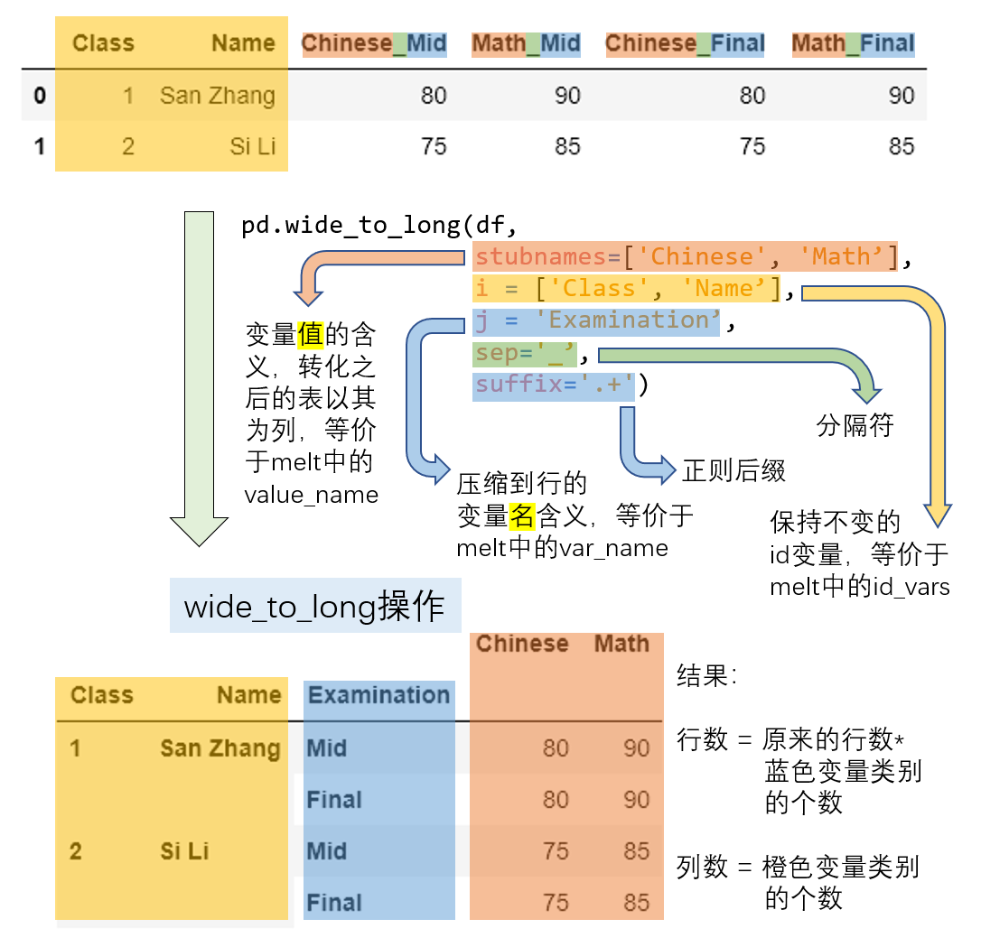
In melt, the column elements compressed into one column can only represent a single level of meaning, namely values_name. If the column labels encode crossed categories - say midterm versus final and Chinese versus math - you may want to expand the Grade corresponding to values_name into two columns, one for Chinese scores and one for math scores, compressing only the midterm/final information. That is when wide_to_long is needed.
| |
| Class | Name | Chinese_Mid | Math_Mid | Chinese_Final | Math_Final | |
|---|---|---|---|---|---|---|
| 0 | 1 | San Zhang | 80 | 90 | 80 | 90 |
| 1 | 2 | Si Li | 75 | 85 | 75 | 85 |
| |
| Chinese | Math | |||
|---|---|---|---|---|
| Class | Name | Examination | ||
| 1 | San Zhang | Mid | 80 | 90 |
| Final | 80 | 90 | ||
| 2 | Si Li | Mid | 75 | 85 |
| Final | 75 | 85 |
The transformation is shown in the figure below; elements belonging to the same concept are marked in matching colors:
Here is a more involved case: take the result of the multi-column pivot operation from the previous section (which created a multi-level index) and use wide_to_long to restore its original shape. This uses the str.split function from Chapter 8; for now, simply think of it as splitting a series on a given delimiter.
| |
| Grade | rank | |||
|---|---|---|---|---|
| Class | Name | Subject_Examination | ||
| 1 | San Zhang | Chinese_Mid | 80 | 10 |
| Chinese_Final | 75 | 15 | ||
| Math_Mid | 90 | 20 | ||
| Math_Final | 85 | 7 | ||
| 2 | Si Li | Chinese_Mid | 85 | 21 |
| Chinese_Final | 65 | 15 | ||
| Math_Mid | 92 | 6 | ||
| Math_Final | 88 | 2 |
| |
| Class | Name | Examination | Subject | Grade | rank | |
|---|---|---|---|---|---|---|
| 0 | 1 | San Zhang | Mid | Chinese | 80 | 10 |
| 1 | 1 | San Zhang | Final | Chinese | 75 | 15 |
| 2 | 2 | Si Li | Mid | Chinese | 85 | 21 |
| 3 | 2 | Si Li | Final | Chinese | 65 | 15 |
| 4 | 1 | San Zhang | Mid | Math | 90 | 20 |
| 5 | 1 | San Zhang | Final | Math | 85 | 7 |
| 6 | 2 | Si Li | Mid | Math | 92 | 6 |
| 7 | 2 | Si Li | Final | Math | 88 | 2 |
II. Reshaping Indexes
1. stack and unstack
Chapter 2 introduced swapping levels within an index using swaplevel or reorder_levels. What follows concerns exchanges $\color{red}{\text{between row and column indexes}}$ - that is, between the row and column indexes. Because such an exchange changes the dimensions of the DataFrame, it is a reshaping operation. The four reshaping functions in the first section differ in that they convert $\color{red}{\text{elements}}$ of one or more columns and the $\color{red}{\text{column indexes}}$ into each other, rather than converting indexes into one another.
unstack moves a row index level into the column index, as in this simple example:
| |
| col_1 | col_2 | |||
|---|---|---|---|---|
| A | cat | big | 1.0 | 1.0 |
| dog | small | 1.0 | 1.0 | |
| B | cat | big | 1.0 | 1.0 |
| dog | small | 1.0 | 1.0 |
| |
| col_1 | col_2 | ||||
|---|---|---|---|---|---|
| big | small | big | small | ||
| A | cat | 1.0 | NaN | 1.0 | NaN |
| dog | NaN | 1.0 | NaN | 1.0 | |
| B | cat | 1.0 | NaN | 1.0 | NaN |
| dog | NaN | 1.0 | NaN | 1.0 | |
The main parameter of unstack is the level to be moved; by default the innermost level is converted and placed at the innermost level of the column index. Several levels can be converted at once:
| |
| col_1 | col_2 | ||||
|---|---|---|---|---|---|
| big | small | big | small | ||
| A | cat | 1.0 | NaN | 1.0 | NaN |
| dog | NaN | 1.0 | NaN | 1.0 | |
| B | cat | 1.0 | NaN | 1.0 | NaN |
| dog | NaN | 1.0 | NaN | 1.0 | |
| |
| col_1 | col_2 | |||||||
|---|---|---|---|---|---|---|---|---|
| A | B | A | B | |||||
| big | small | big | small | big | small | big | small | |
| cat | 1.0 | NaN | 1.0 | NaN | 1.0 | NaN | 1.0 | NaN |
| dog | NaN | 1.0 | NaN | 1.0 | NaN | 1.0 | NaN | 1.0 |
As with the uniqueness requirement in pivot, unstack requires the combination of $\color{red}{\text{the row-index level converted into a column index}}$ and $\color{red}{\text{the row-index level that is retained}}$ to be unique. For instance, making the first two column labels identical breaks uniqueness and raises an error:
| |
| col_1 | col_2 | |||
|---|---|---|---|---|
| A | cat | big | 1.0 | 1.0 |
| big | 1.0 | 1.0 | ||
| B | cat | big | 1.0 | 1.0 |
| dog | small | 1.0 | 1.0 |
| |
ValueError('Index contains duplicate entries, cannot reshape')
The opposite of unstack is stack, which pushes a column index level down into the row index; its usage is entirely analogous.
| |
| A | B | |||
|---|---|---|---|---|
| cat | dog | cat | dog | |
| big | small | big | small | |
| index_1 | 1.0 | 1.0 | 1.0 | 1.0 |
| index_2 | 1.0 | 1.0 | 1.0 | 1.0 |
| |
| A | B | ||||
|---|---|---|---|---|---|
| cat | dog | cat | dog | ||
| index_1 | big | 1.0 | NaN | 1.0 | NaN |
| small | NaN | 1.0 | NaN | 1.0 | |
| index_2 | big | 1.0 | NaN | 1.0 | NaN |
| small | NaN | 1.0 | NaN | 1.0 | |
| |
| A | B | |||
|---|---|---|---|---|
| index_1 | cat | big | 1.0 | 1.0 |
| dog | small | 1.0 | 1.0 | |
| index_2 | cat | big | 1.0 | 1.0 |
| dog | small | 1.0 | 1.0 |
2. The Relationship Between Aggregation and Reshaping
Of all the functions described above, every one except pivot_table, which aggregates, leaves the number of values unchanged before and after reshaping; only their presentation changes. The group-aggregation operation from the previous chapter necessarily counts as a special kind of reshaping, since it creates new row and column indexes, but aggregation collapses several original values into one and therefore changes the number of values. That is the essential difference between grouped aggregation and the reshaping functions.
III. Other Reshaping Functions
1. crosstab
crosstab occupies an awkward position, since everything it can do can also be done with pivot_table. By default it counts how often combinations of elements occur - a count operation. For example, to count the frequency of each school and transfer-status combination in the learn_pandas dataset:
| |
| Transfer | N | Y |
|---|---|---|
| School | ||
| Fudan University | 38 | 1 |
| Peking University | 28 | 2 |
| Shanghai Jiao Tong University | 53 | 0 |
| Tsinghua University | 62 | 4 |
This is equivalent to the following way of writing crosstab, where aggfunc is the aggregation parameter:
| |
| Transfer | N | Y |
|---|---|---|
| School | ||
| Fudan University | 38.0 | 1.0 |
| Peking University | 28.0 | 2.0 |
| Shanghai Jiao Tong University | 53.0 | NaN |
| Tsinghua University | 62.0 | 4.0 |
An equivalent result can also be obtained with pivot_table. Since we are counting combinations here, whichever column is passed to values has no effect on the outcome:
| |
| Transfer | N | Y |
|---|---|---|
| School | ||
| Fudan University | 38.0 | 1.0 |
| Peking University | 28.0 | 2.0 |
| Shanghai Jiao Tong University | 53.0 | NaN |
| Tsinghua University | 62.0 | 4.0 |
The difference between the two functions is now clear: crosstab receives an actual series in that position, whereas pivot_table receives the name of a column in the calling table; passing a series to pivot_table raises an error.
Beyond the default count, all aggregation strings and custom functions returning a scalar are available. For instance, to compute the mean height for each combination:
| |
| Transfer | N | Y |
|---|---|---|
| School | ||
| Fudan University | 162.043750 | 177.20 |
| Peking University | 163.429630 | 162.40 |
| Shanghai Jiao Tong University | 163.953846 | NaN |
| Tsinghua University | 163.253571 | 164.55 |
2. explode
explode expands the elements of a column vertically. The cell to be exploded must hold one of list, tuple, Series, np.ndarray.
| |
| A | B | |
|---|---|---|
| 0 | [1, 2] | 1 |
| 1 | my_str | 1 |
| 2 | {1, 2} | 1 |
| 3 | 0 3 1 4 dtype: int64 | 1 |
| |
| A | B | |
|---|---|---|
| 0 | 1 | 1 |
| 0 | 2 | 1 |
| 1 | my_str | 1 |
| 2 | 1 | 1 |
| 2 | 2 | 1 |
| 3 | 3 | 1 |
| 3 | 4 | 1 |
3. get_dummies
get_dummies is one of the important functions for feature construction: it turns categorical features into indicator variables. For example, converting the grade column into indicators marks the column for a student’s grade with 1 and all others with 0:
| |
| Freshman | Junior | Senior | Sophomore | |
|---|---|---|---|---|
| 0 | 1 | 0 | 0 | 0 |
| 1 | 1 | 0 | 0 | 0 |
| 2 | 0 | 0 | 1 | 0 |
| 3 | 0 | 0 | 0 | 1 |
| 4 | 0 | 0 | 0 | 1 |
IV. Exercises
Ex1: The U.S. Illicit Drug Dataset
Here is a dataset about illicit drugs in the United States, where SubstanceName, DrugReports denote the substance name and the number of reports, respectively:
| |
| YYYY | State | COUNTY | SubstanceName | DrugReports | |
|---|---|---|---|---|---|
| 0 | 2011 | KY | ADAIR | Buprenorphine | 3 |
| 1 | 2012 | KY | ADAIR | Buprenorphine | 5 |
| 2 | 2013 | KY | ADAIR | Buprenorphine | 4 |
- Reshape the data into the following form:
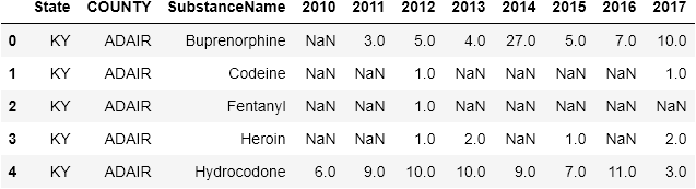
- Restore the result of Question 1 to the original table.
- For each
State, compute the total number of reports per year, withState, YYYYas the column and row indexes respectively. Implement this in two different ways - withpivot_tableand withgroupbyplusunstack- and reflect on the connection between them.
Ex2: A Special wide_to_long Approach
Functionally, melt should be a special case of wide_to_long in which stubnames has only one entry. Use wide_to_long to produce the df_melted from the melt section. (Hint: add a suitable prefix to the column names.)
| |
| Class | Name | Chinese | Math | |
|---|---|---|---|---|
| 0 | 1 | San Zhang | 80 | 80 |
| 1 | 2 | Si Li | 90 | 75 |