
Pandas Time Series Data
| |
I. Basic Objects in Time Series
Time series are a familiar concept in daily life, but a concrete temporal event can be described from several different object perspectives. Suppose you must be in class at 8 a.m. on Monday, September 7, 2020, and the class ends at 10 a.m. that same morning. What time concepts does this involve?
First, there are timestamps (Date times): the two points ‘2020-9-7 08:00:00’ and ‘2020-9-7 10:00:00’ represent the moments when class begins and ends; in
pandasthey are calledTimestamp. A series of timestamps can form aDatetimeIndex, and once placed in aSeries, theSerieshas dtypedatetime64[ns], ordatetime64[ns, tz]when a time zone is involved, where tz is short for timezone.Second, there are time deltas (Time deltas): the duration of the class. Subtracting two
Timestampobjects gives a time delta, represented in pandas byTimedelta. Likewise, a series of time deltas forms aTimedeltaIndex, and placing it in aSerieschanges theSeriesdtype totimedelta64[ns].Third, there are time spans (Time spans): class continues throughout the interval from 8 to 10, represented in
pandasbyPeriod. Similarly, a series of time spans forms aPeriodIndex, and placing it in aSerieschanges theSeriesdtype toPeriod.Fourth, there are date offsets (Date offsets): suppose you only know that class starts at 8 a.m. on the first Monday of September, without knowing the exact date; a type is needed for such cases. Again, if you want the 30th working day after September 7, 2020, a time delta cannot solve the problem, and so
DateOffsetappears inpandas.pandashas no dedicated storage type for a column of date offsets, for a simple reason: such needs are unusual, and generally we only need to apply one uniform special offset to a batch of time features.
This simple example makes it easy to summarize the table from the official documentation:
| Concept | Single-element type | Array type | pandas dtype |
|---|---|---|---|
| Date times | Timestamp | DatetimeIndex | datetime64[ns] |
| Time deltas | Timedelta | TimedeltaIndex | timedelta64[ns] |
| Time spans | Period | PeriodIndex | period[freq] |
| Date offsets | DateOffset | None | None |
Because the time-span objects Period/PeriodIndex are not used very often, they will not be covered here; the discussion is confined to timestamp series, time-delta series, and date offsets.
II. Timestamps
1. Constructing and Attributes of Timestamp
A single timestamp is created with pd.Timestamp; in general, common date formats can all be converted successfully:
| |
Timestamp('2020-01-01 00:00:00')
| |
Timestamp('2020-01-01 08:10:30')
The individual values can be obtained through year, month, day, hour, min, second:
| |
2020
| |
1
| |
1
| |
8
| |
10
| |
30
In pandas, the smallest precision of a timestamp is the nanosecond ns; using 64-bit storage, the representable time range can be calculated approximately as follows:
The range representable by timestamps can be obtained via pd.Timestamp.max and pd.Timestamp.min; as you can see, the span in years is indeed about the result computed above:
| |
Timestamp('2262-04-11 23:47:16.854775807')
| |
Timestamp('1677-09-21 00:12:43.145225')
| |
585
2. Generating Datetime Series
A group of timestamps can form a time series, generated with to_datetime and date_range. to_datetime converts an object column of timestamp-formatted values into a datetime64[ns] time series:
| |
0 2019-10-05
1 2019-09-04
2 2019-09-12
3 2020-01-03
4 2019-11-06
Name: Test_Date, dtype: datetime64[ns]
In the rare cases where the timestamp format does not match, you can force a match with format:
| |
DatetimeIndex(['2020-01-01', '2020-01-03'], dtype='datetime64[ns]', freq=None)
Note that because a list rather than a pandas Series was passed above, the result is a DatetimeIndex; to obtain a datetime64[ns] series, convert explicitly with Series:
| |
0 2020-01-01
1 2020-01-03
dtype: datetime64[ns]
There is also a to_datetime operation that concatenates several time columns of a table into a time series; the column names must match the following time-keyword names:
| |
0 2020-01-01 10:30:20
1 2020-01-02 20:50:40
dtype: datetime64[ns]
date_range generates a continuous, regularly spaced sequence of times. Its important parameters are start, end, freq, periods, denoting the start time, end time, interval, and number of timestamps. When any three of the four are given, the remaining one is determined. Note that if the start or end date is an endpoint, it is included:
| |
DatetimeIndex(['2020-01-01', '2020-01-11', '2020-01-21'], dtype='datetime64[ns]', freq='10D')
| |
DatetimeIndex(['2020-01-01', '2020-01-11', '2020-01-21', '2020-01-31',
'2020-02-10', '2020-02-20'],
dtype='datetime64[ns]', freq='10D')
| |
DatetimeIndex(['2020-01-01 00:00:00', '2020-01-12 14:24:00',
'2020-01-24 04:48:00', '2020-02-04 19:12:00',
'2020-02-16 09:36:00', '2020-02-28 00:00:00'],
dtype='datetime64[ns]', freq=None)
The freq parameter here is closely tied to DateOffset objects; its concrete use will be introduced in Section IV.
[Exercise]
Timestamp defines a value attribute whose integer value is the number of nanoseconds between 1970-01-01 00:00:00 and the given timestamp. Use this attribute to write a function that randomly generates dates within a given date range.
[END]
Finally, a method for changing a series’ sampling frequency is asfreq, which performs an operation similar to reindex according to a given freq:
| |
2020-01-01 0.393911
2020-01-03 0.703650
2020-01-05 0.650046
2020-01-07 0.726203
2020-01-09 0.126783
dtype: float64
| |
2020-01-01 0.393911
2020-01-02 NaN
2020-01-03 0.703650
2020-01-04 NaN
2020-01-05 0.650046
Freq: D, dtype: float64
| |
2020-01-01 00:00:00 0.393911
2020-01-01 12:00:00 NaN
2020-01-02 00:00:00 NaN
2020-01-02 12:00:00 NaN
2020-01-03 00:00:00 0.703650
Freq: 12H, dtype: float64
[NOTE]
As mentioned earlier, datetime64[ns] can essentially be understood as a large integer. For a series of this type you can use max, min, mean to obtain the maximum timestamp, the minimum timestamp, and the “average” timestamp.
[END]
3. The dt Object
Just as cat, str are defined on category, string series for categorical and text data, a dt object is defined on time-series-typed series to support many time-series operations. For datetime64[ns], these operations fall roughly into three groups: extracting time-related attributes, testing whether timestamps satisfy conditions, and rounding.
The common attributes of the first group include date, time, year, month, day, hour, minute, second, microsecond, nanosecond, dayofweek, dayofyear, weekofyear, daysinmonth, quarter, where daysinmonth, quarter denote the number of days in the month and the quarter respectively.
| |
0 2020-01-01
1 2020-01-02
2 2020-01-03
dtype: object
| |
0 00:00:00
1 00:00:00
2 00:00:00
dtype: object
| |
0 1
1
2
2 3
dtype: int64
| |
0 31
1 31
2 31
dtype: int64
Among these attributes, dayofweek is frequently used; it returns the day of the week, with Monday as 0, Tuesday as 1, and so forth:
| |
0 2
1 3
2 4
dtype: int64
In addition, month_name, day_name return English month and weekday names; note that they are methods rather than attributes:
| |
0 January
1 January
2 January
dtype: object
| |
0 Wednesday
1 Thursday
2 Friday
dtype: object
The second group of tests mainly checks whether a date is the first or last day of a month/quarter/year:
| |
0 True
1 False
2 False
dtype: bool
| |
0 False
1 False
2 False
dtype: bool
The third group, rounding, includes round, ceil, floor, whose common parameter is freq; common values include H, min, S (hour, minute, second), and all available freq values can be found here.
| |
0 2020-01-01 20:35:00
1 2020-01-01 21:20:00
2 2020-01-01 22:05:00
dtype: datetime64[ns]
| |
0 2020-01-01 21:00:00
1 2020-01-01 21:00:00
2 2020-01-01 22:00:00
dtype: datetime64[ns]
| |
0   2020-01-01 21:00:00
1   2020-01-01 22:00:00
2   2020-01-01 23:00:00
dtype: datetime64[ns]
| |
0   2020-01-01 20:00:00
1   2020-01-01 21:00:00
2   2020-01-01 22:00:00
dtype: datetime64[ns]
4. Slicing and Indexing Timestamps
In general, timestamp series serve as indexes. To select a sub-series of timestamps, the first approach combines the dt object with boolean conditions; the other uses slicing, which is common for consecutive timestamps. Here are a few examples:
| |
2020-01-01    0
2020-01-02    1
2020-01-03    1
2020-01-04    0
2020-01-05    0
Freq: D, dtype: int32
Example 1: The first or last day of each month
| |
2020-01-01    0
2020-01-31    1
2020-02-01    1
2020-02-29    1
2020-03-01    0
dtype: int32
Example 2: Weekends
| |
2020-01-04    0
2020-01-05    0
2020-01-11    1
2020-01-12    0
2020-01-18    0
dtype: int32
Example 3: Extracting a single day’s value
| |
0
| |
0
Example 4: Extracting July
| |
2020-07-01    1
2020-07-02    1
2020-07-03    0
2020-07-04    1
2020-07-05    0
Freq: D, dtype: int32
Example 5: From early May to July 15
| |
2020-05-01    1
2020-05-02    1
2020-05-03    1
2020-05-04    1
2020-05-05    1
Freq: D, dtype: int32
| |
2020-07-11    1
2020-07-12    1
2020-07-13    1
2020-07-14    1
2020-07-15    1
Freq: D, dtype: int32
III. Time Deltas
1. Generating Timedeltas
As noted in Section I, a time delta can be understood as the difference between two timestamps, and it can also be constructed with pd.Timedelta:
| |
Timedelta('1 days 00:25:00')
| |
Timedelta('1 days 00:25:00')
| |
Timedelta('1 days 00:25:00')
The main way to generate a time-delta series is pd.to_timedelta, whose dtype is timedelta64[ns]:
| |
0 0 days 00:04:34
1 0 days 00:04:20
2 0 days 00:05:22
3 0 days 00:04:08
4 0 days 00:05:22
Name: Time_Record, dtype: timedelta64[ns]
Like date_range, a time-delta series can also be generated with timedelta_range; the two have identical parameters:
| |
TimedeltaIndex(['0 days 00:00:00', '0 days 00:06:00', '0 days 00:12:00'], dtype='timedelta64[ns]', freq='6T')
| |
TimedeltaIndex(['0 days 00:00:00', '0 days 00:08:20', '0 days 00:16:40'], dtype='timedelta64[ns]', freq=None)
As with timestamp series, a dt object is also defined for Timedelta series. The attributes defined above include days, seconds, mircroseconds, nanoseconds, which return the corresponding features of the time delta. Note that seconds here does not mean the total number of seconds, but the seconds left after taking the remainder over days:
| |
0 274
1 260
2 322
3 248
4 322
Name: Time_Record, dtype: int64
If you want the total seconds rather than the remainder over days, use total_seconds
| |
0    274.0
1    260.0
2    322.0
3    248.0
4    322.0
Name: Time_Record, dtype: float64
As with timestamp series, the rounding functions can also be used on the dt object:
| |
0   0 days 00:05:00
1   0 days 00:04:00
2   0 days 00:05:00
3   0 days 00:04:00
4   0 days 00:05:00
Name: Time_Record, dtype: timedelta64[ns]
2. Timedelta Operations
Time deltas support three common kinds of operations: multiplication by a scalar, addition and subtraction with timestamps, and addition, subtraction, and division with other time deltas:
| |
Timedelta('2 days 00:00:00')
| |
Timedelta('2 days 00:00:00')
| |
Timestamp('2020-01-02 00:00:00')
| |
Timestamp('2019-12-31 00:00:00')
All of these operations carry over to time-delta series:
| |
TimedeltaIndex(['5 days', '10 days', '15 days', '20 days', '25 days'], dtype='timedelta64[ns]', freq='5D')
| |
0    0 days
1    2 days
2    6 days
3   12 days
4   20 days
dtype: timedelta64[ns]
| |
TimedeltaIndex(['0 days 12:00:00', '1 days 10:00:00', '2 days 08:00:00',
                '3 days 06:00:00', '4 days 04:00:00'],
               dtype='timedelta64[ns]', freq=None)
| |
DatetimeIndex(['2020-01-02', '2020-01-03', '2020-01-04', '2020-01-05',
               '2020-01-06'],
              dtype='datetime64[ns]', freq='D')
| |
DatetimeIndex(['2020-01-02', '2020-01-04', '2020-01-06', '2020-01-08',
               '2020-01-10'],
              dtype='datetime64[ns]', freq=None)
IV. Date Offsets
1. Offset Objects
A date offset is a special time delta tied to the calendar. Recall the two questions from Section I: how to find the date of the first Monday in September 2020, and how to find the 30th working day after September 7, 2020.
| |
Timestamp('2020-09-07 00:00:00')
| |
Timestamp('2020-10-19 00:00:00')
As the examples show, Offset objects are defined in pd.offsets. Using + yields the nearest following date, whereas - yields the nearest preceding date:
| |
Timestamp('2020-08-03 00:00:00')
| |
Timestamp('2020-07-27 00:00:00')
| |
Timestamp('2020-09-30 00:00:00')
For the common date offsets, consult the documentation here. Among the Offset objects listed there, one special case deserves mention: CDay, whose holidays, weekmask parameters filter custom dates and weekdays respectively. The former takes a list of dates to exclude; the latter takes a weekday string made of three-letter abbreviations and keeps only the weekdays appearing in that string:
| |
2020-01-08    2
2020-01-09    3
2020-01-10    4
2020-01-11    5
Freq: D, dtype: int64
| |
[Timestamp('2020-01-10 00:00:00'),
 Timestamp('2020-01-10 00:00:00'),
 Timestamp('2020-01-15 00:00:00'),
 Timestamp('2020-01-15 00:00:00')]
In the example above, n means adding one CDay. The first date in dr is 20200108, but since the next day 20200109 is excluded and 20200110 is a valid Friday, it becomes 20200110; the later dates are handled similarly.
[CAUTION] Do Not Use Partial Offsets
Due to several bugs in the current version, do not use Offset objects below the Day level, such as Hour, Second; use the corresponding Timedelta objects instead.
[END]
2. Offset Strings
Earlier we noted that the freq of date_range may take an Offset object, and in pandas nearly every Offset object is bound to an offset string (frequencies strings/offset aliases) that can be used in its place. Here are some common examples.
| |
DatetimeIndex(['2020-01-01', '2020-02-01', '2020-03-01'], dtype='datetime64[ns]', freq='MS')
| |
DatetimeIndex(['2020-01-31', '2020-02-29', '2020-03-31'], dtype='datetime64[ns]', freq='M')
| |
DatetimeIndex(['2020-01-01', '2020-01-02', '2020-01-03', '2020-01-06',
               '2020-01-07', '2020-01-08', '2020-01-09', '2020-01-10'],
              dtype='datetime64[ns]', freq='B')
| |
DatetimeIndex(['2020-01-06', '2020-01-13', '2020-01-20', '2020-01-27'], dtype='datetime64[ns]', freq='W-MON')
| |
DatetimeIndex(['2020-01-06'], dtype='datetime64[ns]', freq='WOM-1MON')
The strings above are equivalent to using the following Offset objects:
| |
DatetimeIndex(['2020-01-01', '2020-02-01', '2020-03-01'], dtype='datetime64[ns]', freq='MS')
| |
DatetimeIndex(['2020-01-31', '2020-02-29', '2020-03-31'], dtype='datetime64[ns]', freq='M')
| |
DatetimeIndex(['2020-01-01', '2020-01-02', '2020-01-03', '2020-01-06',
               '2020-01-07', '2020-01-08', '2020-01-09', '2020-01-10'],
              dtype='datetime64[ns]', freq='B')
| |
DatetimeIndex(['2020-01-06', '2020-01-13', '2020-01-20', '2020-01-27'], dtype='datetime64[ns]', freq='C')
| |
DatetimeIndex(['2020-01-06'], dtype='datetime64[ns]', freq='WOM-1MON')
[CAUTION] A Note on Time Zones
For the development of the various time objects, besides Python’s built-in datetime module, pandas also uses dateutil, largely to handle time zones. As is well known, China has no daylight saving time, but some countries do, making a day relatively 23/24/25 hours long — the relativedelta — so Offset and Timedelta objects may yield different results for the same problem. The rules are fairly complex, parts of the official documentation are inaccurate, and a unified correction is hard because many Offset components are involved. This tutorial therefore disregards time-zone handling entirely; if you are interested in discussing time-zone offsets, you can contact me or see the discussion here.
[END]
V. Rolling Windows and Grouping in Time Series
1. Rolling Windows
A rolling window for time series replaces the window size with the freq keyword. Here is a concrete example: the stock market has an indicator called BOLL, composed of three lines — the middle band, upper band, and lower band — computed respectively as the N-day mean line, the N-day mean plus two N-day standard deviations, and the N-day mean minus two N-day standard deviations. Using a rolling object, the BOLL indicator for N=30 can be written as follows:
| |
2020-01-01   -1
2020-01-02   -2
2020-01-03   -1
2020-01-06   -1
2020-01-07   -2
Freq: B, dtype: int32
| |
[<matplotlib.lines.Line2D at 0x26941924dc8>]
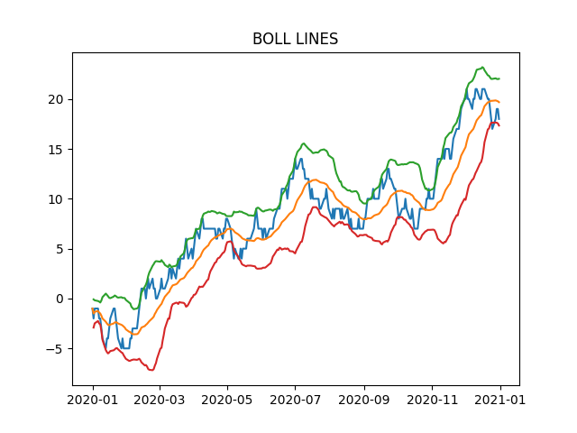
For the shift function, when applied to a series indexed by datetime64, freq can be specified to control the shift:
| |
2020-02-20   -1
2020-02-21   -2
2020-02-22   -1
2020-02-25   -1
2020-02-26   -2
dtype: int32
In addition, applying diff to a datetime64[ns] series yields a timedelta64[ns] series, which lets users conveniently examine the intervals of an ordered time series:
| |
0 2020-01-01
1 2020-01-02
2 2020-01-03
3 2020-01-06
4 2020-01-07
dtype: datetime64[ns]
| |
0      NaT
1   1 days
2   1 days
3   3 days
4   1 days
dtype: timedelta64[ns]
2. Resampling
The resampling object resample is similar in use to the grouping object groupby in Chapter 4; the former is a grouping object designed for grouped computation on time series.
For example, compute the mean every 10 days for the series above:
| |
2020-01-01   -2.000000
2020-01-11   -3.166667
2020-01-21   -3.625000
2020-01-31   -4.000000
2020-02-10   -0.375000
Freq: 10D, dtype: float64
If no built-in handler is available, you can define one with apply:
| |
2020-01-01    3
2020-01-11    4
2020-01-21    4
2020-01-31    2
2020-02-10    4
Freq: 10D, dtype: int32
In resample, special care is needed with group boundary values. By default, the starting value is computed by adding freq from midnight 00:00:00 of the date corresponding to the minimum timestamp up to the largest timestamp not exceeding that minimum; this timestamp then becomes the start. Each freq is accumulated as a split point for grouping, with intervals left-closed and right-open. Let’s construct an uneven example:
| |
2020-01-01 08:26:35   -1
2020-01-01 08:27:52   -1
2020-01-01 08:29:09   -2
2020-01-01 08:30:26   -3
2020-01-01 08:31:43   -4
Freq: 77S, dtype: int32
The first group below starts at 08:24:00, obtained by adding 72 increments of freq=7 min to midnight; adding another freq would exceed the series’ minimum timestamp 08:26:35:
| |
2020-01-01 08:24:00   -1.750000
2020-01-01 08:31:00   -2.600000
2020-01-01 08:38:00   -2.166667
2020-01-01 08:45:00    0.200000
2020-01-01 08:52:00    2.833333
Freq: 7T, dtype: float64
Sometimes users want groups formed by starting at the series’ minimum timestamp and incrementing freq; in that case set the origin parameter to start:
| |
2020-01-01 08:26:35   -2.333333
2020-01-01 08:33:35   -2.400000
2020-01-01 08:40:35   -1.333333
2020-01-01 08:47:35    1.200000
2020-01-01 08:54:35    3.166667
Freq: 7T, dtype: float64
Note that the returned index is usually the first timestamp of a group, but for the seven values M, A, Q, BM, BA, BQ, W it is the last timestamp of the corresponding interval:
| |
2020-01-31    0.451613
2020-02-29    0.448276
2020-03-31    0.516129
2020-04-30    0.566667
2020-05-31    0.451613
Freq: M, dtype: float64
| |
2020-01-01    0.451613
2020-02-01    0.448276
2020-03-01    0.516129
2020-04-01    0.566667
2020-05-01    0.451613
Freq: MS, dtype: float64
VI. Exercises
Ex1: The Solar Radiation Dataset
Here is a dataset about solar radiation:
| |
| Data | Time | Radiation | Temperature | |
|---|---|---|---|---|
| 0 | 9/29/2016 12:00:00 AM | 23:55:26 | 1.21 | 48 |
| 1 | 9/29/2016 12:00:00 AM | 23:50:23 | 1.21 | 48 |
| 2 | 9/29/2016 12:00:00 AM | 23:45:26 | 1.23 | 48 |
- Merge
Datetime, Timeinto a single time columnDatetime, set it as the index, and then sort. - The intervals between records are obviously inconsistent. Solve the following problems:
- Find the three groups of timestamps corresponding to the three largest intervals.
- Is there an approximate range within which the vast majority of intervals fall? If so, draw a histogram of the interval seconds for samples in that range, with
bins=50.
- Find the
Seriescorresponding to the following metrics:
- The 6-hour rolling correlation between temperature and radiation
- The mean temperature series for the time interval in which each observation lies, split at 3 a.m., 9 a.m., 3 p.m., and 9 p.m.
- The radiation amount 6 hours before each observation (generally not an exact timestamp; use the radiation of the nearest timestamp)
Ex2: The Fruit Sales Dataset
Here is a record of daily fruit sales in 2019:
| |
| Date | Fruit | Sale | |
|---|---|---|---|
| 0 | 2019-04-18 | Peach | 15 |
| 1 | 2019-12-29 | Peach | 15 |
| 2 | 2019-06-05 | Peach | 19 |
- Compute the following metrics:
- The ratio of grape sales in the first half of each month (through the 15th) to those in the second half
- The total sales of pears on the last day of each month
- The total sales of pears on the last working day of each month
- The mean sales of apples over the last five days of each month
- For each month, compute the mean number of records for each fruit from Monday through Sunday; the outer level of the row index is the fruit name, the inner level the month, and the column index the weekday.
- Compute, by day, the mean apple sales over a forward-looking 10-working-day window, filling non-working days with the previous working day’s result.